Showing posts with label abstract mathematics. Show all posts

Engineering as the theory of airlocks

In this post, I will describe four different objects or systems, from seemingly unrelated concrete situations. They achieve purposes that are in some sense analogous, and they act by mechanisms that are in some sense analogous. You are recommended to figure out, by yourself, before I explain, what this "sense" is, what the precise connection between these concrete notions are, what the purpose of this article is, and why I am asking you to figure all this out for yourself (and recursion thereof).

The vacuum's bodyguard

We wish to maintain a vacuum uninterrupted in a room. However, we also wish to allow people to enter this room, and worry that when we open the door for people to enter, air will rush in along with them.

It is clear that if we open the door, anything outside will enter. So we need to make sure there is no air directly outside the door. So we install a small chamber (with its own door) right outside this door, so that both doors are never simultaneously open, and the chamber has a mechanism to pump out any air in it.

The security guard

Perhaps the title of the previous example was already too revealing. But yes, we do have a trivial analogy to a security guard who filters out uninvited visitors, or to a biological containment room, or a shoe stand outside a temple.

The AI box

You have created a General AI, and decided to put it in a box, a Faraday cage to prevent it from talking to anyone.

(You have also put Eliezer Yudkowsky in a box, to drown out the horrified yelling.)

But you want to be able to talk with the AI, but worry that in opening the door to the box, you will give the AI a brief period of time to communicate with the outside world.

So you come up with the idea of putting the box in another box, so that both boxes are never open at the same time. You enter the outside box, close it, then open the inside box and talk to the AI.

Please allow passengers to alight before boarding.

You see an elevator (or a train), and observe that alighting an boarding passengers keep crashing into each other instead of letting one happen before the other.

You're a busybody, but a creative one, so instead of taking pictures of it and expressing outrage on Facebook, you decide to come up with a solution.

It seems like a difficult problem at first -- a door is fundamentally symmetric, it doesn't care about what direction you're moving in.

But well, a door is fundamentally symmetric, but that doesn't mean systems of doors have to be.


You create intermediary entry and exit chambers as above (you really only need an exit chamber, I just like the symmetrical-looking drawing), and operate the doors in the sequence as labeled above: (initially all closed) open 1, close 1, open 2, close 2, open 3, close 3.

Variable swaps

You're writing some code, and want to interchange the values of two variables x and y, for some reason. Unfortunately, writing x=y; y=x will just set both of them to the original value of y, because the first assignment eliminated the original value of x.

So you create a third variable z, and write z=x; x=y; y=z (or alternatively if you want something that looks symmetric, use a "quad swap": x1=x; y1=y; x=y1; y=x1).

(Similarly, exchanging the positions of two physical objects.)

The wolf, the goat and the cabbage

This is a classic, of course. A farmer must carry a wolf, goat and cabbage across a river. The boat holds only one of these items at a time, and neither the wolf and goat, or goat and cabbage, can be left unattended together at once.

(Why does a farmer need a wolf? To attack his competition's goats and establish a monopoly, of course. But that's not important to us.)

The solution, you may recall, is to first take the goat across, then come back and take the wolf across, bring back the goat and take the cabbage across, then come back for the goat.

Sanitation protocols

You have two pieces of dirty cutlery to clean: a bowl and a spoon. You can only hold/wash one item at a time, and the spoon must be kept in a bowl if it is not being held. Solution: you introduce a new piece of cutlery, a clean bowl, to store the spoon after it's washed, as the dirty bowl is being washed.

(The original example involved washing a car and a carpark, but there are too many additional complications there like how you move a dirty car from one place to another. Nonetheless, you are welcome to spend a few seconds thinking about this alternative example, and exactly how you would "abstract away" the irrelevant complications.)

You're eating food from a large container with a spoon, but do not wish to contaminate it as you re-insert the spoon. Solution: You transfer the quantity you wish to eat to another container and eat from that.

You're showering in a public toilet, and you must wear clothes while going into and out of the toilet -- but that will reintroduce germs to your person. Solution: You bring a change of clothes.

You must touch the tap again after you wash your hands to shut it off, thus reintroducing germs to your hands. Solution: You observe the following protocol -- switch on the tap, clean your hands, clean the tap, clean your hands again, switch off the tap.

Scaffolding in Photoshop

You're editing an image. You want to edit something-something using something-something-else but then the two things will mix, or something like that. So Photoshop allows you to make multiple layers which you can view in overlay, then delete the ones you used as scaffolding.


Do you see the connection?

In all these examples, we needed to enforce a specific desired mechanism of transport or action, across a door that was fundamentally symmetric. And the solution involved creating a temporary chamber to do some sorting.

In the first few examples, this was obvious, but notions of "transport", "doors" and "chambers" became increasingly more abstract. In the last example, the "temporary chamber" was the first time you washed your hands.

These are all applications of the same principle, the principle of the airlock.

You see the same principle appear, for instance with semiconductor technology and logic gates, public key encryption, and escrows (aka "How do I know you won't run off with the money and that you know I won't run off with the money?").

In a sense, the airlock is the fundamental unit of the modern world -- in the sense that engineering is the theory of airlocks. The principle of the airlock underlies any task of imposing a specific order on something disorderly or chaotic, to exercise control for a specific purpose, over the natural, unaligned, nihilistic behaviour of nature.


But enough about that. We're not here to serenade the airlock.

Suppose someone asked you the question "Does an airlock really exist? Or is it just an intellectual tool?" Surely each specific concrete manifestation of the airlock -- the security guard, or the change of clothes -- exists. But the abstraction?

But no one would actually ask that. It is a meaningless question -- it is something in the grammatical form of a question, but the possible answers "yes, the airlock really exists" and "no, the airlock doesn't really exist" don't mean anything, if you don't precisely specify the meaning of "exist".

Except when it isn't an airlock, but instead the set of imaginary numbers, people actually do ask that question.

Like the airlock is the abstraction of the idea of setting up mechanisms to impose an order to something symmetric, the imaginary number (at least multiplicatively) is the abstraction of the idea of right-angle rotations.

It is pretty common to answer "imaginary numbers exist in the same way that the number 3 exists" or "imaginary numbers exist in the same way that triangles exist". But instead, I propose we answer "imaginary numbers exist in the same way that the airlock exists".

Motivating ring theory, domains with integer-polynomial analogies

When you were first introduced to polynomial long division, you were struck by how a process that worked for integers worked for abstract polynomials. Integer division seemed rather "specific" -- focused on details like the resulting quotient having to be an integer -- and it seems bizarre that even the notion of integer division could be generalized beyond the integers.

It's not like integer division is just polynomial division with $x=10$ or something -- the results of the division are different, because integer division does not assume a base of 10.

But polynomial division also focuses on an analogous detail: the resulting quotient having to be a polynomial. And the essential lesson of mathematics, and the idea of abstract mathematics, is that serious analogies are the sign of abstraction.

So what makes polynomials and integers similar -- in what sense are they similar? -- that we can perform a "long division" algorithm on them?

And you know: this is not the only analogy between integers and polynomials either. Here's a list, with a general "abstract" phrasing that works for both integers and polynomials:
  • Division with remainder: For any $a,b$, there is some "unique" representation $a=qb+r$, where "uniqueness" is with respect to the property that $r<b$ (this $<$ ordering on the integers refers to the the ordering of the absolute value, and on the polynomials refers to the degree).
  • Bezout's identity: For any $a, b$, the set $\{\lambda a + \mu b\}$ is precisely the multiples of $\mathrm{gcd}(a, b)$.
  • Unique factorization: For any $a$, there exists a unique representation $a=p_1\dots p_n$ among $p_i$ that are "prime" ("irreducible") in the sense of not having any further factors. Well, is that really true? Not exactly: prime numbers can be factored with $-1$s and $1$s, and irreducible polynomials can be factored with constant polynomials. Well, this caveat has to do with stuff having itself as a factor, e.g. $x-2=(1/2)\cdot(2)\cdot(x-2)$ or $37=(-1)\cdot(-1)\cdot 1\cdot 37$. This means the other elements of this "factorization of the prime number" multiply to 1/are each "invertible" ("units"). So we should say we have unique factorization is "up to units". 
  • Greatest common divisors: For any $a, b$, there is a $\delta$ that divides both and is divided by all $d$ that divide both $a$ and $b$ (note that the term "divides" can exist in more generality than the assumptions of "division with remainder").
Well, the first thing we observe is that we should assume the existence of some notions of addition, subtraction and multiplication -- these seem to be the "fundamental" structures present among integers and polynomials (as opposed to e.g. rational numbers, rational functions which also require division or natural numbers which don't have subtraction). 

We will omit discussing the properties of these operations for now, as we don't yet have enough to motivate them on. 

Next, each of these discussed properties can be considered as special axioms for special cases of rings, domains where specific important theorems hold -- we call them, respectively: 
  • Euclidean domain: The ring is equipped with a natural number-valued magnitude function $\|\cdot\|:R\to\mathbb{Z}^{\ge 0}$, called the Euclidean function. For all $a,b$ in $R$ with $b$ non-zero (intuit out this condition), there exist $q, r$ with $\|r\|<\|b\|$ such that $a=qb+r$. 
  • Principal Ideal Domain: A ring where all ideals (additive subgroups invariant under multiplication by a ring element) are principal (a set of multiples of a generating element). Another abstraction is a "Bezout domain", which only requires that linear combinations of principal ideals are principal, but a PID should be seen as a more "natural" generalization.
  • Unique factorization domain: A ring where every element has a unique factorization into irreducibles, modulo multiplication by a unit. 
  • GCD domain: A ring in which any two elements has a GCD. 
(Quick comments on why the Euclidean function must map to the naturals: in fact, they could map to any "well-ordered set" (a totally ordered set in which every subset has a least element). The reason why this property is needed -- why we can't, e.g. map to the nonnegative reals -- is to ensure Euclid's algorithm terminates.)

The abstractions of the basic theorems about integers and polynomials occur as relationships between these domains. As it turns out, we will see that:
\[{\rm{ED}} \Rightarrow {\rm{PID}} \Rightarrow {\rm{UFD}} \Rightarrow {\rm{GCD}}\]
Before that, though, we can already play with some basic results we'd like, to get a feel of what axioms about ring addition and multiplication we should assume.

E.g.
  • What should $\|0\|$ equal? Prove that 0 must have the least magnitude of any ring element, making up the axioms you need on the fly. You should require: additive identity, additive inverse, additive associativity.
  • Try to prove some obvious results regarding Bezout's identity, like with $a$ and $b$ equal. You should require: left-distributivity, right-distributivity
  • Consider generalizations of two-element properties, like the Bezout identity, to multiple elements. You should require additive associativity, multiplicative associativity, additive commutativitymultiplicative commutativity.
Well, to be honest these all seem like fairly elementary properties that would be useful outside the cases of these special domains. Out of the following properties:
  1. Left-distributivity
  2. Right-distributivity
  3. Additive associativity
  4. Additive identity
  5. Additive inverse
  6. Additive commutativity
  7. Multiplicative associativity
  8. Multiplicative identity
  9. Multiplicative commutativity
  10. Multiplicative inverse
10 is not a ring axiom (because integers and polynomials don't have it). 1-7 essentially always are. 8 sometimes is, but not if you want e.g. the even numbers to be a ring. 9 typically isn't, although this is once again mostly just a matter of convention -- you can't really "see" that non-commutative rings appear often enough to justify their classification of rings, etc.

Presumably 6 (additive commutativity) is hardest to see the importance of, but it's relevant to note the relationships between these axioms. In fact, it is fairly simple to show that 1, 2 and 8 imply 6 (consider $(1+1)(x+y)$). As a result, addition -- the operation that multiplication distributes over -- is just generically seen as commutative.

Another important property often seen in algebraic problems is the ability to factor to find roots, i.e. to say that if $ab=0$, either $a$ or $b$ should be 0. This is known as an integral domain. The full sequence of inclusions, as we will see, is actually given by:
\[{\rm{ED}} \Rightarrow {\rm{PID}} \Rightarrow {\rm{UFD}} \Rightarrow {\rm{GCD}} \Rightarrow {\rm{ID}} \Rightarrow {\rm{Ring}}\]
The broader point of all this is that you should start often thinking of a lot of basic mathematical facts in the language of abstract algebra -- what kind of ring/domain is this result valid in? etc. -- because this is the most general setting in which a result is valid in, and you know exactly what it is "saying", i.e. what implies what. 

Abstracting our abstractions: "limits of cones", universal properties

The last article, Abstracting some categorical definitions, saw the same kind of construction repeated over and over: given some diagram, we'd ask for an object with morphisms to or from that diagram (demanding that the diagram commute) -- such an object would be a "candidate" for our construction, and we'd then ask for the "maximum" or "minimum" among such constructions.

That this notion appears so frequently makes sense. It's really a generalisation of the notions of initial and final topologies, and comes from the notion that an object is defined by its morphisms to or from other objects, and that we're interested in constructions that are unique up to isomorphism.

So consider some diagram in $\mathcal{C}$. As we will later see, this is formally a "functor" (morphism between categories) from an indexing category $\mathcal{I}$ to $\mathcal{C}$ -- denote it as $X:\mathcal{I}\to\mathcal{C}$.
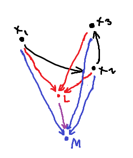
We define a cone to $\mathcal{C}$ as an object $M$ together with morphisms $m_i:M\to X_i$ such that it commutes with the existing diagram (formally, such that for every morphism $f:i\to j$ in $\mathcal{I}$, we have $F(f)\circ m_i=m_j$).
Now this necessarily represents an object with "more information than each $X_i$" -- so we're interested in the "infimum" of these cones, the one with the least information, the one to which there exists a morphism from any other cone. The limsup of cones, if you will:
We define the limit $(L,\ell_i)$ of the diagram to be a cone such that for any cone $(M,m_i)$ to the diagram, $\exists!\ u:M\to L$ such that the diagram commutes, i.e. $m_i=\ell_i\circ u$ forall $i$.
The above diagram commutes, and the purple morphism is unique.
And the dual notion is also observed, a liminf:
We define a co-cone from $\mathcal{C}$ as an object $\overline{M}$ together with morphisms $\overline{m}_i:X_i\to \overline{M}$ such that it commutes with the existing diagram (formally, such that for every morphism $f:i\to j$ in $\mathcal{I}$, we have $\overline{m}_j\circ F(f)=\overline{m}_i$).
We define the co-limit $(\overline{L},\overline{\ell}_i)$ of the diagram to be a cone such that for any cone $(\overline{M},\overline{m}_i)$ to the diagram, $\exists!\ u:\overline{L}\to \overline{M}$ such that the diagram commutes, i.e. $\overline{m}_i=u\circ\overline{\ell}_i$ forall $i$.
The below diagram commutes, and the purple morphism is unique.
Alternatively, the limit and colimit may be characterised as the final object in the category of cones and the initial object in the category of co-cones respectively (check that this makes sense).

Examples:
Diagrams captioned by their limits.

(empty diagram)
Limit: final object
Co-limit: initial object

(discrete diagram)
Limit: product
Co-limit: co-product

This answers the difficult cases of the empty product (it's just the final object) and the power (use the constant functor).
(parallel diagram)
Limit: equaliser
Co-limit: co-equaliser

Exercises: Do some examples to convince yourself of the following ideas:
  • Even if there are a bunch of morphisms in the diagram, the limit of the diagram talks fundamentally about the product of the "starting" objects of the diagram (think of: $X\rightarrow Y\leftarrow Z$, etc.).
  • If your original diagram has non-commuting features, the limit of the diagram talks about equalisers of these features (think of: parallel diagram, reverse-parallel diagram $\leftrightharpoons$, other cycles, a diagram with non-trivial automorphisms).
  • Adding commuting stuff doesn't change the limit (i.e. the limit of $X\to Y\to Z$ is the same if you add another morphism $X\to Z$).


Universal objects and comma categories

You may have noticed that images and coimages cannot be written as limits and colimits (do you see why?). We made a fairly specific specialisation when defining limits/colimits that doesn't really have to do with our "limsup/liminf" intuition -- we insisted we had morphisms either from or to the diagram, whereas we could in general have a more complicated property.

In general, instead of dealing with the category of cones, we could deal with some other category (called the comma category) and discuss its initial and final objects instead.

The key insight regarding this generalisation is as follows: one can see the limit as a construction in the category $\mathcal{C}^{\mathcal{I}}$ of diagrams in $\mathcal{C}$ of a certain shape $\mathcal{I}$. The limit object (which is an object in $\mathcal{C}$) can be "upgraded" to that category as the constant diagram (an element of $\mathcal{C}^{\mathcal{I}}$ that maps every node in the diagram shape to the same object in $\mathcal{I}$) (this "upgrading" is called the diagonal functor $\Delta: \mathcal{C}\to\mathcal{C}^\mathcal{I}:=\lambda M.\ (\lambda i.\ M)$) with a morphism to the object of $\mathcal{C}^\mathcal{I}$ we're actually taking the limit of.

So more generally, we can consider some category other than $\mathcal{C}^\mathcal{I}$, and a more general functor than $\Delta$, in order to formalise a more general notion of being a limiting object. We make the following definition:
We define the final morphism from a functor $F:\mathcal{C}\to\mathcal{D}$ to an object $D\in\mathcal{D}$ as a morphism $\ell:F(L)\to D$ such that for any morphism $m:F(M)\to D$, there $\exists!\ u: M\to L$ such that the diagram commutes, i.e. $m=\ell\circ F(u)$.
You may observe that $F$ generalised $\Delta$, $\mathcal{D}$ is the generalisation of the "category of diagrams", and the final morphism generalises the limit (with $L$ being the limit "object" in $\mathcal{C}$). Analogously we define, generalising the colimit:
We define the initial morphism to a functor $F:\mathcal{C}\to\mathcal{D}$ from an object $D\in\mathcal{D}$ as a morphism $\overline{\ell}:D\to F(\overline{L})$ such that for any morphism $\overline{m}:D\to F(\overline{M})$, there $\exists!\ u: \overline{L}\to \overline{M}$ such that the diagram commutes, i.e. $\overline{m}=F(u)\circ\overline{\ell}$.
These terms "final morphism" and "initial morphism" are not to be confused with the morphisms to and from an initial object or a final object, that we defined previously. Typically, these terms are used in neither context -- one simply says "universal morphism" to/from $D$ from/to $F$; and in the previous context, one simply says morphisms to a final object/from an initial object.

In general, these morphisms are referred to as universal morphisms or universal objects.

(By the way: the term "universal property" is just used to refer to the property of being initial or terminal or whatever.)

This notion can easily be restated as follows: given an object $D\in\mathcal{D}$ and a functor $F:\mathcal{C}\to\mathcal{D}$, one can construct the following:
The comma category $[F\to D]$ is a category whose objects are the morphisms $m:F(M)\to D$, and whose morphisms from $m_1\to m_2$ are given by morphisms $u:M_1\to M_2$ such that the diagram commutes, i.e. such that $m_1=m_2 \circ F(u)$.
The cocomma category $[D\to F]$ is a category whose objects are the morphisms $m:D\to F(M)$ and whose morphisms from $m_1\to m_2$ are given by morphisms $u:M_1\to M_2$ such that the diagram commutes, i.e. such that $m_2=F(u)\circ m_1$
Then a final morphism is the final object in the comma category, and an initial morphism is the initial morphism is the initial object in the cocomma category. If $\mathcal{D}=\mathcal{C}^{\mathcal{I}}$ (i.e. is a diagram category) and $F$ is the diagonal functor, then the comma category is the category of cones, and the cocomma category is the category of cocones.

One might dislike the asymmetry between $F$ and $D$ and decide to go a step further, generalising $D$ to another functor. So given two functors $F:\mathcal{A}\to\mathcal{D}$ and $G:\mathcal{B}\to\mathcal{D}$, we can construct:
The comma category $[F\to G]$ is a category whose objects are the morphisms $m:F(M)\to G(N)$ and whose morphisms from $m_1\to m_2$ are given by morphisms $u:M_1\to M_2,\ v: N_1\to N_2$ such that the following diagram commutes:
The previous definition of comma and cocomma categories then occur when $\mathcal{B}$ and $\mathcal{A}$ respectively are replaced by a singleton (and $D$ is the only object in their image in $\mathcal{D}$).


Examples: free group, image

Abstracting some categorical definitions

Before making any interesting definitions, we need to get something over with: the notions of injective and surjective homomorphisms do not really generalise very nicely to category theory -- the closest definitions are:
A morphism $f:X\to Y$ is a monomorphism if for distinct morphisms $g$ to $X$, $f\circ g$ are distinct.
A morphism $f:X\to Y$ is an epimorphism if for distinct morphisms $g$ from $Y$, $g\circ f$ are distinct.
One may check that all injective homomorphisms are monomorphisms and that all surjective homomorphisms are epimorphisms -- but it's not too hard to see that they are not equivalent. Concrete counter-examples exist even in simple categories like abelian groups.

If anyone has any motivation or insightful explanation of monomorphisms and epimorphisms, let me know. For example, are the non-injective monomorphisms (e.g. the quotient map $\mathbb{Q}\to\mathbb{Q}/\mathbb{Z}$) actually interesting or just something we need to get used to?

There are also related notions:
A morphism $f:X\to Y$ is a section if it has a left-inverse ("retraction"), i.e. a morphism $g:Y\to X$ such that $g\circ f=1_X$.
A morphism $f:X\to Y$ is a retraction if it has a right-inverse ("section"), i.e. a morphism $g:Y\to X$ such that $f\circ g=1_Y$.
It's clear that all sections are injective morphisms (and thus monomorphisms), and all retractions are surjective morphisms (and thus epimorphisms). Of course, these intermediaries are not category-theoretic.

One may define an isomorphism, denoted $f:X\leftrightarrow Y$, as a morphism that is both a section and a retraction. Here are some theorems about it:
An isomorphism has a two-sided inverse morphism.
Given $g_1\circ f=1_X$, $f\circ g_2=1_Y$ -- by considering $g_1\circ f\circ g_2$, we see that $g_1=g_2$.
A morphism that is both a monomorphism and a retraction is an isomorphism.
Since $f$ is a retraction, $f \circ g = {1_Y}$ -- so $f \circ g \circ f = f$. Left-cancelling (since $f$ is a monomorphism), $g\circ f = 1_Y$, thus $f$ is a section.
A morphism that is both a section and a epimorphism is an isomorphism.
Analogous to above.


Subobjects

In our minds, a sub-object is a subset that also carries the structure of that category -- in other words, it's isomorphic to another object in that category.

It's natural to identify the subobjects of $X$ then with injections (or rather monomorphisms) into $X$ (not with the domains of the injections, as they may have multiple embeddings into $X$). But the identification is not one-to-one -- multiple injections may have the same image. In general, two monomorphisms $g_1:S_1\hookrightarrow X$, $g_2:S_2\hookrightarrow X$ having the same image is an equivalence relation, expressible as:
$$\exists i:S_1\leftrightarrow S_2,\ g_1=g_2\circ i$$
So we identify the equivalence classes of monomorphisms into an object with its subobjects.

An alternate motivation for our definition of a subobject comes from the subspace topology (and vice versa), which is defined in terms of continuous inclusion maps. Of course, in our definition here, we allow the subspace topology to be any topology that allows an injective continuous map to the space, but the standard definition in topology asks for the coarsest such topology (i.e. the "least continuous" such map). Later, we will study some refined definitions of a lot of ideas here that may apply better to specific categories.


Quotient objects

The natural way to think of quotient objects in category theory is in terms of the first isomorphism theorem, which states that the quotient objects are the images of surjections from the object -- kinda "dual" to how subobjects are the images of injections into the object (keep this notion of "duality" in mind).

You might be afraid that this kind of defeats the point, since we'd like to eventually prove the First Isomorphism Theorem in category theory. Well, we'll do so with some other more category-specific definition of quotients, etc. so the First Isomorphism Theorem would simply be a demonstration that these two definitions are equivalent.

But once again, just identifying the quotient objects with epimorphisms overcounts them -- a single quotient can map to multiple different isomorphic things. So, as before, we write down an equivalence relation between epimorphisms from $X$: two epimorphisms $g_1:X\twoheadrightarrow Q_1$, $g_2:X\twoheadrightarrow Q_2$ are equivalent if:
$$\exists i: Q_1\leftrightarrow Q_2,\ g_2=i\circ g_1$$
So we identify these equivalence classes of epimorphisms as the quotient objects of an object $X$.


Products

One can take inspiration from the product topology, and think of the product of some objects as the object with the "least information" that still allows morphisms to each object. So we define:
Given a collection $X_i$ of objects, we define their product $\prod X_i$ as a collection of morphisms $\pi_i:X\to X_i$ such that:
  1. For any other collection of morphisms $\pi'_i:X'\to X_i$, $\exists! u: X' \to X$ such that $\pi'_i=\pi_i\circ u$.
Question: what does the empty product look like? This definition seems a bit bad for this purpose. We'll develop some more general machinery in the next article or so.


Sums (aka "coproducts")

Shockingly enough, the "opposite" or "dual" of the above. Direct sums of vector spaces can be seen as the "smallest possible" (i.e. embedding into most possible things, i.e. having most possible information) vector space permitting morphisms from each vector space. Another example would be the disjoint union of sets. Perhaps this is even clearer with the free product of groups, where the free product is the object with the "most information possible" arising from your groups.
Given a collection $X_i$ of objects, we define their sum $\coprod X_i$ as a collection of morphisms $\varpi_i:X_i\to X$ such that:
  1. For any other collection of morphisms $\varpi'_i:X_i\to X'$, $\exists! u: X \to X'$ such that $\varpi'_i=u\circ \varpi_i$.
Because of its "dual" appearance to the product (which we will soon see described more generally), the sum is often known as the "coproduct".


We'll now start to list subobjects and quotient objects related to a morphism. Here's a convenient cheat-sheet: the following diagram is commutative. (dotted lines are zero morphisms, which we will define shortly)

(play with it!)


Images

Next, let's think about the image of a morphism $f$. Once again, we can identify an image with a monomorphism, so we're really looking for a subobject consisting of monomorphisms $g$ with the same image as $f$. So we want an $e:I\to Y$ such that there exists a morphism $f_I: X\to S$ with $f=e\circ f_I$ -- but this is not enough, $I$ may be "too big" (it may contain elements that map to $Y$ not in the image), so we define:
A monomorphism $e:I\hookrightarrow Y$ is the image of a function $f:X\to Y$ if:
  1. $\exists f_I:X\to I, f=e\circ f_I$
  2. For any $e':I'\to Y$ and $f_{I'}:X\to I'$ such that $f=e'\circ f_{I'}$, there $\exists! u:I\to I', e=e'\circ u$.
This relies on the following key lemma of course: the images of $f$ form a subobject. This follows straightforwardly from the second condition.


Zero objects

Many categories have the notion of a zero element in an object -- groups have identities, vector spaces have zero vectors, and let's not talk about rings and fields. And some, like topological spaces, don't.

But we can't talk about elements of an object in category theory. But perhaps the examples above give you an idea -- we have seen trivial groups and trivial vector spaces. Objects comprising only of the zero element -- let's call them zero objects. So maybe we can talk about the images of morphisms from these trivial objects to other objects, and they would represent zero elements.

The idea behind a zero element is that it is "privileged" in some sense -- a morphism must preserve it. Furthermore, every object contains a zero element, so there must always be morphism from the zero object to any object. These criteria fixes a unique morphism from the zero object to any given object. In fact, this idea is captured by the following definition.
A universal object or initial object $I$ is an object such that for any object $X$ in the category, there is a unique morphism $I\to X$.
But there is also another idea behind the notion of a zero object, that it carries the "minimum information" compatible with the category's structure. Recall our interpretation of a morphism as something that either retains or discards information -- mapping an object to a zero object means discarding "as much information as possible".
A final object $F$ is an object such that for any object $X$ in the category, there is a unique morphism $X\to I$.
Finally, a zero object is defined as an object that is both initial and final.

Perhaps a bit surprising at first (but trivially easily), but we can in fact see that the initial and final objects are respectively unique up to (unique) isomorphism -- just consider the unique morphisms between the two objects. The reason it's kinda incredible that we can do this in full generality, is that e.g. we can immediately see that the trivial ring is not an initial object (because the ring of integers is), because it can't be mapped to anything, something that seems like a technicality at first glance arising from the fact that 1 must be preserved by ring homomorphisms.

But if you think about it, the category theoretic argument also comes from the same fact -- it comes from the fact that you can't map the ring of integers to its own zero element, because that doesn't preserve 1. But if you didn't mandate that ring homomorphisms preserve the multiplicative identity, then the ring of integers would no longer be an initial object.


Zero morphisms, kernels and equalizers

When defining a kernel of $f:X\to Y$, we're looking for a subobject of $X$ that maps to the zero element in $Y$. Since in category theory, a subobject is an injection (from an object we'd typically view as isomorphic to the subobject), we're looking for a monomorphism (subobject) $k$ that composes with $f$ to give us a morphism that maps everything to the zero element, whatever that means.

OK -- so what does it mean? What's a morphism that maps everything to the zero element? Recall that we're thinking of the "zero element" as the image of a morphism from the zero object (which really means we're identifying it with a subobject, i.e. an equivalence class of monomorphisms). So we can associate with our desired morphism $o:X\to Y$ the morphism from $X$ to the zero object, which then embeds into $Y$ -- so we define the zero morphism as their composition:
$$o:=X\to O\to Y$$
Where $O$ is the zero object.
$$\dots$$
There is an alternate, more general definition of a zero morphism for categories without a zero object that nonetheless caputres the notion of a zero element.

Here's an alternate way to think about morphisms from and to a zero object. An initial morphism is essentially the "least surjective homomorphism possible". A final morphism is essentially the "least injective homomorphism possible". These are in line with our understanding of the zero object as the "smallest possible" object, or the one that contains the least information.

In line with the way we've thought of injectivity and surjectivity when defining monomorphisms and epimorphisms, we make the following definitions.
A morphism $f:X\to Y$ is an initial morphism (or right-zero morphism, or coconstant morphism) if for any $g,h: Y\to V$, $g\circ f = h \circ f$.
A morphism $f:X\to Y$ is an final morphism (or left-zero morphism, or constant morphism) if for any $g,h: W\to X$, $f\circ g = f\circ h$.
(Exercise: Check that the morphism from an initial object and the morphism to a final object satisfy this property.)

Further, one may observe that for $l:X\to Y$ final and $r:Y\to Z$ initial, $r\circ l$ is both an initial and a final morphism. So the right general notion of a "morphism that maps everything to the zero element" is a "a morphism that is both initial and final", or a zero morphism.

$$\dots$$
Anyway, we're obviously interested in monomorphisms $k$ to $X$ such that $f\circ k=o$. But these don't all represent the kernel -- they could represent subobjects smaller than the kernel. So we define the kernel as follows:
A monomorphism $k:K\hookrightarrow X$ is the kernel of $f:X\to Y$ if
  1. $f\circ k=o_{KY}$
  2. For any $k':K'\hookrightarrow X$ such that $f\circ k'=o_{K'Y}$, $\exists! u:K'\to K, k\circ u = k'$.
More generally:
Given morphisms $f_i:X\to Y$, their equaliser is a monomorphism $k:X\hookrightarrow X$ such that:
  1. $f_i\circ k$ are equal for all $i$.
  2. For any $k':K'\hookrightarrow X$ such that $f_i\circ k'$ are equal for all $i$, $\exists! u:K'\to K, k\circ u = k'$.
The kernel can then be understood as the equaliser of a morphism with the zero morphism.

Of course, these definitions lie on a key lemma: the kernel/equaliser is a subobject -- i.e. that for two kernels $k_1:K_1\to X$ and $k_2:K_2\to X$, there $\exists i:K_1\leftrightarrow K_2, k_1=k_2\circ i$ -- this follows straightforwardly from the second condition in the definition.


Cokernels, coimages and quotienting by a subobject

I once said that one of the points of learning linear algebra was as an introduction to ideas that appear repeatedly throughout algebra. Here's where we really see this in action.

Recall the notion of a left null space $\mathrm{ker}(f^T)$ from linear algebra -- it sort-of represented the "space of constraints" on the image of a morphism, in that it was the orthogonal complement of the image $\mathrm{im}(f)$ in the co-domain. It represents the stuff that the image can't fall into -- or tying back into our understanding of morphisms as things that "cannot create information that wasn't already present in the domain", it represents the information the morphism hasn't created (whether or not it could have), a measure of non-surjectivity.

Well, "orthogonal complement of the image" is not something restricted to vector spaces -- we can understand it more generally, as a quotient. Interestingly, it would then no longer be a subobject, which I suppose is reasonable -- we don't really have a notion right now of what a transpose morphism is in a general category.

In general, though, the quotient we're looking for is not $Y/\mathrm{im}(f)$ -- clearly, that wouldn't exist in a lot of important categories, e.g. groups. That's only true in categories that seem "abelian" in some sense. Perhaps this is unsurprising, because we're thinking of the cokernel as "the information that the morphism has not created", and information is more than just elements of the set.

So the appropriate way to generalise "a quotient by the image" is to look at a quotient object of the codomain $Y$ (which, recall, is an epimorphism from $Y$) that composes with $f$ to produce the zero morphism. But dually in the case of the kernel, we must make sure that our quotient is the full, "most universal" one:
Given a function $f:X\to Y$, we define its cokernel as an epimorphism $\bar{k}:Y\to\bar{K}$ such that:
  1. $\bar{k}\circ f = o_{X\bar{K}}$
  2. For any other $k':Y\to\bar{K}'$, there $\exists! u:\bar{K}\hookrightarrow\bar{K}'$ such that $k'=u\circ k$.
Once again, the latter property shows that the equivalence class of these epimorphisms is indeed a quotient object.

In fact, this "composition forms the zero morphism" notion is the generalisation of the "quotient by an object" notion, or of the so-called exact sequence below. Generally, given a subobject $S$ given by some monomorphisms $s:S\to X$, the epimorphisms $q:X\to Q$ that always compose with these monomorphisms to form the zero morphism $q\circ s = o_{SQ}$ define the quotient $X/S$, if they are a quotient object.

$$O \to \ker f \to X \overset f \longrightarrow Y \to \operatorname{coker} f \to O$$
Oh, and an exact sequence is exactly the idea behind quotienting by an object.

$$\dots$$
Now recall the notion of a row space $\mathrm{im}(f^T)$. Once again, the row space is best interpreted as a quotient object of $X$ (in the case of linear algebra, the quotient by $\mathrm{ker}(f)$). But constructing it in terms of the kernel would clearly be quite complicated -- and perhaps not generally so useful. A better, more "general" approach is to think of an element of the row space as an equivalence class of elements that are mapped to the same element. So we define:
Given a function $f:X\to Y$, we define its coimage as an epimorphism $\bar{e}:X\twoheadrightarrow \bar{I}$ such that:
  1. $\exists f_{\bar{I}}:\bar{I}\to Y, f = f_{\bar{I}}\circ \bar{e}$
  2. For any other epimorphism $\bar{e}':X\twoheadrightarrow \bar{I}'$ and $f_{\bar I'}:\bar{I}'\to Y$ such that $f = f_{\bar I'}\circ \bar{e}'$, there $\exists! u: \bar{I}'\to\bar{I}, \bar{e}=u\circ \bar{e}'$
Which is again clearly a quotient object.

Introduction to category theory: a second-abstraction

When we first started talking about abstraction, we did so by observing the analogies between mathematical objects, such as integers and polynomials, the unit circle and remainders, etc. We spent the rest of the Abstract Algebra I series figuring out why these seemingly unrelated objects had similar behaviour -- what the fundamental properties were that resulted in this behaviour, and making these properties the "axioms" of various abstract algebraic structures.

But you may have later observed that even these various algebraic structures have analogies. For starters, every algebraic structure has the notion of homomorphisms -- things that commute with "structure". Then you have analogous object constructions, like trivial objects, product objects and quotient objects. And then you have the really neat stuff -- stuff like "normal subgroups are the kernels of group homomorphisms" vs. "ideals are the kernels of ring homomorphisms", etc. And perhaps most usefully of all, we've seen that some analogies themselves, such as between features of Lie groups and features of Lie algebras, might have a simpler and more abstract basis than the specific constructions of the theory.

You would be justified to believe that these analogies spring fro;m some shared principles -- and you would be justified to believe that these shared principles ought to be abstracted.

That much like how mathematical objects were found to have similar properties, and we'd categorise them as groups and rings and vector spaces and whatever -- these categories of objects too could have similar properties.

So this will be our approach: without stating the axioms beforehand and only general notions of what a category is and what a homomorphism (or "morphism" in category theory) is, we will try to prove theorems we know about specific categories like groups, for general categories -- and see what axioms we'll need.

(This, by the way, is called reverse mathematics. We've done this often here whenever dealing with something we must be rigorous about, e.g. in Topology.)

And the real idea we should have at the back of our heads is that we should stop thinking of groups, etc. as "sets with additional structure". They're really generalisations of sets, and homomorphisms are generalisations of functions. (I won't go here into exactly what I mean, but a good article to get your head wrapped around this is Sigma fields are Venn diagrams, for an illustration of how measurable functions, the morphisms in the measurable spaces category, are a "generalisation of functions".) So we won't try to force our objects to be sets and give them elements, or force our morphisms to be functions -- they will just be dots and arrows satisfying some axioms. This will require a bit of thinking, e.g. defining kernels without talking about identity elements.

Let's start.

What even are pure and applied math, anyway?

Not really a serious post.

I see the words "pure math" and "applied math" used a lot, and there seem to be some completely distinct meanings of the phrases:
  1. Formal math and informal math -- you can certainly approach things like summing divergent series completely formally (follow the link for proof!), and I'm sure you could in principle be hand-wavy with category theory. So this is really about the method with which you do mathematics, not the field itself. An example of where you see this is the distinction between analysis and calculus (well, a distinction -- sometimes calculus is defined specifically as having to do with differentials and integrals while analysis is a broader field).
  2. Abstract math and concrete math -- this really has multiple levels: category theory, abstract mathematics, mathematics, science, engineering, specific numerical calculation. The line is often drawn either before or after "mathematics".
  3. Theoretical and applied -- closely related to the previous point, differing by the purely social question of the purpose of the study.
  4. Everything else vs statistics -- I think this arises from a conflation between statistics and applied/concrete statistics. Statistics can really be a totally formal field of mathematics or even abstract mathematics, but I guess people often fail to draw the distinction (unlike, say, between "differential equations" and "applied differential equations in engineering").
  5. Algebra vs everything else -- Perhaps a result of the fact that analysis and geometry often restrict to handling special concrete objects like the real and complex numbers.
I guess the reason these distinctions are often taken as synonymous is that they're quite correlated. As you get more abstract, you may feel a stronger obligation to be more formal to make sure you haven't missed out on some so-called pathological cases (although I think it's perfectly possible to develop intuition for such pathological situations, see e.g. my e^(-1/x) article, or the topology series). When working for an applied purpose, it may not be useful to be too formal, for practical constraints.

The correlation really lines up with the fundamental "purpose of mathematics". The point of having axiomatisations is that someone applying abstract ideas in concrete situations can just check if the axioms are satisfied -- and so you really must formally deduce things from them to make sure you're not making some assumptions specific to one concrete situation that you have in mind.

(Another example of such ambiguity is the distinction between "theoretical science" and "practical science". I've still not figured out if the latter refers to experimental science or applied science, and there isn't even any correlation between the ideas here.)

Supplementary definitions: levels of abstraction

Although we have been able to generalise a lot of our theorems about the topological properties of metric spaces to topological spaces, several others remain out of our reach, and we need to find the right level of abstraction that makes them true -- and we can usually do this by trying to prove the theorem and seeing what it "needs", then if this theorem actually characterises the space, proving the need is equivalent to the theorem.

Separation axioms

We've seen the first one. TFAE:
  • $X$ is a T0/Kolmogorov/distinguishable space.
  • All points in $X$ are distinguishable.
  • For any pair of points, there exists an open set containing exactly one of them.
Now, in metric spaces, statements like "there is a point of a set (or sequence) $S$ in every open neighbourhood of $x$" are equivalent to "there are an infinite number of points of $S$ in every open neighbourhood of $x$", i.e. every open neighbourhood of a limit point of $S$ has infinite points in $S$. The key here is that at any step in the process, an open neighbourhood of $x$ can be constructed that does not contain any of the previous points in the sequence, i.e. there exists an open neighbourhood of $x$ not containing some finite number of points.

This is possible, e.g. if we decide that finite sets are closed (or equivalently singletons are closed). This is an iff -- if a finite set $S$ isn't closed, there are points in $\mathrm{cl}(S)$ that aren't in $S$, but it's impossible for there to be an infinite number of points in $S$ in a neighbourhood of such a point, as $S$ is finite.

Wait, what about for points in $S$ itself -- aren't these all also limit points of $S$? We sneakily changed the definition of limit points from $x\in\mathrm{cl}(S)$ to $x\in\mathrm{cl}(S-\{x\})$, i.e. to exclude sequences that include the point itself. So since excluding a set from a finite set keeps it finite, it is still closed, and thus $x$ is not re-included when you close it (so it is not a limit point at all).

Wait, what about the discrete topology on a finite set? All finite sets are closed, but how could we have an infinite number of anything? The key is that there are no "limit points" of any set. So the only T1 finite spaces are the discrete ones.

Note how this implies a stronger form of T0 -- T0 said that for every pair of points, at least one of them has an open neighbourhood excluding the other. Well, in a T1 space, we can always just remove any finite number of points from an open neighbourhood and it will remain an open neighbourhood -- so in particular, this means that for every pair of points, each has an open neighbourhood excluding the other, or any two points are separated. In fact, this is clearly an iff (take some finite intersections).

The closedness of finite sets has plenty of other implications that match our intuition. You will see some in the list of exercises.

So for now, TFAE:
  • $X$ is a T1/Frechet space.
  • All points in $X$ are separated.
  • For any pair of points, each has an open neighbourhood excluding the other.
  • Each open neighbourhood of a limit point of $S\subseteq X$ contains an infinite number of members of $S$.
  • Finite sets are closed/singletons are closed.
We've seen spaces in which limits are not unique. You might think that topological distinguishability should suffice to have unique limits -- is this right?

Let's go through the proof of the uniqueness of limits on metric spaces. Suppose $f$ has two limits $L_1$ and $L_2$ at $c$. Now does it really suffice that there is a neighbourhood of $L_1$ not containing $L_2$? Not necessarily -- it may be the case that this neighbourhood of $L_1$ intersects every neighbourhood of $L_2$ because there's just that amount of indiscretion around $L_2$. What's important is that there exist disjoint neighbourhoods of $L_1$ and $L_2$.

So the uniqueness of limits is equivalent to the existence of disjoint neighbourhoods for distinct points. This is variously called a Hausdorff space or a T2 space. So TFAE:
  • $X$ is a T2/Hausdorff space.
  • All points in $X$ are separated by neighbourhoods.
  • Any pair of points has a pair of respective neighbourhoods disjoint from each other.
  • Limits of nets/filters are unique.
Here's another obvious fact about the topology of metric spaces: any continuous function $f:S\to\mathbb{R}$ on a closed (not just compact) set $S$ may be extended to a continuous function $F:X\to\mathbb{R}$. The proof of this relies on the ability to "connect" points between the pieces of $S$:


You might think that this just means "having a continuous function between two points", but this is only because of the choice of a one-dimensional space -- in general, the "boundary" of each connected component is not just a finite number of points. What does suffice is that for disjoint closed sets $S$ and $T$ there exists a continuous function $h:X\to\mathbb{R}$ "separating" them, i.e. such that $h(S)=\{0\}$, $h(T)=\{1\}$. Then a bunch of such functions can just be added to $f$ to obtain $F$. This is trivally an iff.

One may try further to "prove" the existence of such a continuous function $h$. Well, on $\mathbb{R}$, we have a notion of a "midpoint" between the endpoints of the closed sets -- we could have the value of $h$ at this point be $1/2$, and then continue the construction for all "Dyadic rational"-points.


In general, we don't really need the notion of a midpoint, but we do need some point with "space around it", i.e. open neighbourhoods of each closed set that don't contain the point. We only need the case where $S$ and $T$ are in a connected component, so this is equivalent to the existence of open neighbourhoods of disjoint closed sets. This is also clearly an iff, as one may consider preimages of open sets in $[0,1]$. Thus TFAE:
  • $X$ is a T4/normal space.
  • Every pair of disjoint closed sets has respective disjoint open neighbourhoods. 
  • Every pair of disjoint closed sets can be separated by a continuous function (Urysohn's lemma).
  • Every continuous map on a closed subset can be extended to a continuous map on $X$ (Tietze's extension theorem).

Countability

We've already seen the first one. TFAE:
  • $X$ is a first-countable space.
  • Every point in $X$ has a countable neighbourhood basis.
  • $\lim_{x\to a}f(x)=L\iff\forall (x_{n\in\mathbb{N}})\to a, f(x_n)\to f(a)$. 
  • Every filter has a corresponding sequence.
Several other cardinality functions can be defined and other axioms of countability can be introduced, e.g. sequantial spaces, separable spaces and second-countable spaces, but we cannot really motivate them at this point. (Second-countability in particular important when dealing with metrisability, integration and related issues, as it gives rise to the notion of "paracompactness".)

For the following statements, find the "least restrictive" level of abstraction necessary, and decide if the property characterises the level (i.e. is it an iff?):
  1. Every subset $S$ is the union of all the closed sets contained in $S$.
  2. Every subset $S$ is the intersection of all the open sets containing $S$.
  3. Every nonempty open set contains a nonempty closed set.
  4. Every point $x$ admits a nested neighbourhood basis, i.e. a neighbourhood basis totally ordered by $\subseteq$.
  5. Closed subset $T$ of a compact space $S$ is compact.
  6. Compact space is closed.
  7. There is no smallest neighbourhood of any point (i.e. $\forall x\in X,\forall N\in N(x), \exists M\in N(x), N\not\subseteq M$).
Solutions:
  1. T1. This is equivalent to asking that every point in $S$ is contained in a closed subset of $S$, which is possible if the singleton is closed. For equivalence, consider a singleton $S$.
  2. T1. Dual to Exercise 1.
  3. T1 suffices, but is not equivalent (e.g. the indiscrete topology or any other topology full of clopen sets). Maybe if you change to proper containment.
  4. First-countability. (both sides of equivalence are clear -- think directed set, etc.)
  5. Any topological space suffices. We need to be careful with the proof here because the notions of closedness and compactness are intuitively very similar. Here it is: any net on $T$ is a net on $S$ and thus has a convergent subnet with limit is in $S$ -- but its limit must also be in $T$ because $T$ is closed.
  6. Hausdorff suffices (probably not equivalent, but who cares). The thing is that in general, even on a compact space, although a convergent sequence may have a convergent subsequence in $S$, it may have other limits outside $S$. But in a Hausdorff space, limits are unique.
  7. "Not Alexandrov". Let's characterise the topologies that do have smallest neighbourhoods -- these are necessarily the ones for which arbitrary intersections of open sets are open, and are called finitely-generated topologies or Alexandrov topologies

Topology I: limits, continuity and homeomorphism, the neighbourhood filter, open sets

The idea of a topology, although often linked to geometry* in some classifications, is perhaps better understood as something that has fundamentally more to do with groups, vector spaces and such. You know, when talking about groups, what we really care about is the structure -- we don't really care if we're dealing with $U(1)$ or $SO(2)$ or $\mathbb{Z}/2\pi\mathbb{Z}$ -- if two groups are isomorphic, they have the same "structure" and it's this structure we care about. We're interested in the properties of the group that are invariant under isomorphism -- these are the "group theoretic" properties.

Anyway -- a group homomorphism $f:G\to H$ is a function that preserves the group structure, or alternatively commutes with multiplication, i.e. $f(x\cdot y) = f(x)\cdot f(y)$ (you might see the "commuting" analogy better if you write $x\cdot y$ as $\mathrm{mult}(x,y)$. Similarly, a vector space homomorphism or "linear transformation" $f:V\to W$ is a function that preserves the linear structure or alternatively commutes with linear combination/commutes with addition and scalar multiplication, i.e. $f(ax+y)=af(x)+f(y)$.

Here's another example: the homomorphisms of order theory are increasing functions. Do you see why?

*: It's not completely unrelated to geometry, though, which as we discussed here is the theory of the invariants of a manifold under some symmetries. Well, symmetries are analogous to isomorphisms, but different -- symmetries form a group, in that the transformation from one state of the manifold to another can be judged to be the "same transformation" as that between two other states, i.e. $gx=y$ and $gx'=y'$. But there is no natural way to "parameterise" group isomorphisms so that you can compose them -- is this what one calls a "groupoid"? I don't know.

In general, commuting means some sort of preservation or non-interference policy. Here's another example: a continuous function $f:X\to Y$ is a function that commutes with the limit, i.e.

$$f\left(\lim_{x\to a}x\right)=\lim_{x\to a}f(x)$$
The properties of a space that are invariant under continuous functions are precisely what encompass the theory of topology -- so a topological homomorphism is a "continuous function", and a topological isomorphism is a continuous function with a continuous inverse or a "homeomorphism". The structure of a topological space is precisely the limit operation. It's not a binary operation like group multiplication $(\cdot):G^2\to G$ or vector addition $(+):V^2\to V$ or a unary function family like scalar multiplication $(\cdot):K\times V\to V$, but an operator family $(\lim):(\mathcal{I}\to X) \to (\mathcal{I}\to X)$ where $\mathcal{I}$ is fixed to be the domain set.

We could also phrase this in an equivalent more natural manner -- a continuous function is one that preserves convergent sequences and their limits ("Cauchy" is incorrect on incomplete spaces, e.g. $1/x$ is continuous on $\mathbb{R}^+$ but maps the Cauchy sequence $(1/n)$ to $(n)$).

Well, our equation above doesn't even make sense for incomplete spaces like $\mathbb{R}^+$ or $\mathbb{Q}$ ($\lim_{x\to a}f(x)$ is not necessarily defined), but we still want to talk about the "topology" of such spaces. In any case, we've talked about spaces without even describing what the objects of the space are, or how the "space" arises from the set (endowing with a metric is too much information that isn't invariant under continuous functions).


How would we generalise the notion of a limit to an arbitrary space? The key is something called a "filter" specifically a "neighbourhood filter". Filters are interesting mathematical objects with wide mathematical applications, but in this context, the idea behind a neighbourhood filter is that we want a sort of "convergence" of a poset of sets to a point. You would recall from basic real analysis that expression $\min(\delta_1,\delta_2)$ and $\max(N_1,N_2)$ are of importance to many theorems -- this is taking the intersection of two neighbourhoods and forming a new one. This leads to the following axioms:

Axioms for the neighbourhood topology
  1. $\forall N\in N(x), x\in N$ (to relate the neighbourhoods to the points themselves)
  2. $\forall N\in N(x), \exists M\in N(x), M\subseteq N\land \forall y\in M, N\in N(y)$ (to ensure the sets are only neighbourhoods to points on their "interior")
  3. $\forall N\in N(x), \forall N' \supseteq N, N' \in N(x)$ (to express the notion of convergence -- we really want a "smallest neighbourhood", but since there is no such thing, we want a sequence of neighbourhoods that get arbitrarily small)
  4. $\forall N_1, N_2\in N(x), N_1\cap N_2\in N(x)$ (the intersection thing)
  5. $\forall x\in X, N(x)\ne\varnothing$ (this is not strictly neceessary, but there is a point without neighbourhoods, you could just remove it from the set and not lose anything topological -- do you see why? -- as it is not topologically related to any other point -- do you see why? -- think about what continuous functions do with them)
The last three are the axioms of a filter, and the first two specify the neighbourhood filter in particular. Then the definition of a limit is:

$$\lim_{x\to a}f(x)=L\iff \forall U\in N(L),f^{-1}(U)\in N(a)$$
And the definition of continuity is:

$$\forall U\in N(f(a)),f^{-1}(U)\in N(a)$$
It's a useful exercise to confirm that with the standard neighbourhoods on $\mathbb{R}$, this reduces to the standard definition of the limit. It's also useful to generalise the standard properties of the limit with this definition -- start with the uniqueness of the limit. You'll see that this axiomatisation really does capture the basic "idea" of the limit.

(If the second axiom is a bit unclear, the point is that the set $[0,1)$ is not the neighbourhood of the point 0 even though it contains it -- a neighbourhood must contain an epsilon-ball around the point. Convince yourself that this is necessary by constructing a situation where $f^{-1}(U)$ is $[0,1)$ but $f$ is discontinuous.)

These axioms are the axioms for a topology defined in terms of neighbourhoods, or a neighbourhood topology -- any choice of neighbourhoods satisfying these axioms define a topology on the underlying set.

The second axiom is appalling with its number of quantifiers, but it gives some solid idea of what a neighbourhood really is -- one can show it's equivalent to $\forall x\in\mathrm{Int}A, \mathrm{Int} A\in N(x)$ (where $\mathrm{Int}A$ is the interior of $A$, the set of points of which $A$ is a neighbourhood), i.e. that $\mathrm{Int}A$ is an open set and thus equivalent to $\forall N\in N(x), \mathrm{Int} N\in N(x)$. It is then easy to see that this implies the notion in our head that "a neighbourhood of a point is a set that contains an open set containing that point".

OK, so we have these (circular!) definitions of neighbourhoods and open sets in terms of each other:

Relationship between neighbourhood topology and "associated" open set topology
  1. An open set is a set that is the neighbourhood of each of its points: $O\in\Phi\iff \forall x \in O, O\in N(x)$
  2. A neighbourhood of a point is a set containing an open set containing the point: $N\in N(x)\iff \exists O\in\Phi, x\in O\subseteq N$
Now, so far we've been starting with neighbourhoods and defining open sets from them with (1) -- and our discussion above shows that this respects (2), but instead, we could start with a definition of topology in terms of open sets and define neighbourhoods from them with (2), then check that it respects (1). So we need to find out what axioms an open set topology must satisfy such that the associated neighbourhoods satisfy the axioms for a neighbourhood topology, and that respects (1) (i.e. such that the open sets arising from these neighbourhoods are the same as the original open sets).

To find these axioms, we'll simply try and "prove" each of the neighbourhood topology axioms and see what axioms we could use on the open sets to do so.

Figuring out the right open set axioms: Part I
  1. We want $x\in N(x)$. But this follows from the definition of the neighbourhood in (2), so no axioms on the open sets are imposed here.
  2. Same as above -- you can trivially confirm that the open set contained in the neighbourhood is the $M$ we want. That these two axioms follow from the definition was the point of the definition (2).
  3. Same as above.
  4. What's the open set around $x$ contained by $N_1\cap N_2$? The simplest answer is $O_1\cap O_2$. So this produces an axiom: open sets are closed under finite intersection
  5. Every point having a neighbourhood is equivalent to every point being contained in an open set
Now to ensure the $\text{open sets}\to \text{neighbourhoods} \to \text{open sets}$ chain ends up where it started -- what this is basically doing is ensuring the converse $\text{neighbourhood topology}\Rightarrow\text{open set topology}$, because we will be able to show that these "open set axioms" will be true for the  the open sets arising from a neighbourhood topology, and the point is to find out what axioms are needed to ensure these are the same as the original open set topology and thus the axioms apply to the original open set topology. Do you see why this is kind of a tricky game? Let's hope it works.

Figuring out the right open set axioms: Part II

The neighbourhoods arising from the open set topology $\Phi$ are $N(x)=\{S\subseteq X\mid\exists O\in\Phi,x\in O\subseteq S\}$. The open sets arising from these are $\Phi' = \{S\subseteq X\mid \forall x\in S, S\in N(x)\}$. Or:

$$\Phi'=\{S\subseteq X\mid \forall x\in S, \exists O\in\Phi, x\in O\subseteq S\}$$
It is clear that $\Phi\subseteq\Phi'$. We want to show the converse, that $\Phi'\subseteq\Phi$, i.e.

$$\forall x\in S, \exists O\in\Phi, x\in O\subseteq S\Rightarrow S\in \Phi$$
Or in English: "if every point in $S$ has an open set around it contained in $S$, then $S$ is an open set". Recognising that $S$ is the union of all the $O$'s, it is easy to show that this is equivalent to: if $O_\lambda$ is an arbitrary family of sets in $\Phi$, then $\bigcup_\lambda O_\lambda \in \Phi$, i.e. open sets are closed under arbitrary union.

The union of every such blue circle you can create is equal to $S$.
So we now have an axiomatisation of topology in terms of open sets, the open sets topology: we have a topology on a set $X$ given by a set of its subsets $\Phi$ satisfying:

Axioms for the open set topology: 1st ed.
  1. Every point is contained in an open set: $\forall x\in X, \exists O\in\Phi, x\in O$.
  2. Closure under finite intersection: $\forall O_1, O_2\in \Phi, O_1\cap O_2\in\Phi$.
  3. Closure under arbitrary union: $\forall (O_\lambda)\in\Phi^\mathcal{I}, \bigcup_\lambda O_\lambda\in\Phi$. 
(Exercise: show that these axioms are implied on the open sets by the neighbourhood topology axioms. This is important, because at least with the finite intersection axiom, we just chose the "simplest axiom" available to us, which was stronger than the actual axiom we required, which was $\forall x\in X, \forall (O_1, O_2 \in \Phi)\ni x, \exists O\in\Phi, x\in O\subseteq O_1\cap O_2$. Well, along with the arbitrary union axiom this implies finite intersection, anyway.)

There's actually a further re-formulation one can make: every point is in an open set is, due to the arbitrary union axiom, equivalent to the universe is an open set. So our final formulation of topology is:

Axioms for the open set topology: 2nd ed.
  1. $X\in\Phi$.
  2. Closure under finite intersection: $\forall O_1, O_2\in \Phi, O_1\cap O_2\in\Phi$.
  3. Closure under arbitrary union: $\forall (O_{\lambda\in\mathcal{I}})\in\Phi^\mathcal{I}, \bigcup_\lambda O_\lambda\in\Phi$. 
Recall that as the fifth axiom of the neighbourhood topology was optional -- $X\in\Phi$ is similarly optional -- without it, the topology would basically just be a topology over the union of all open sets. But you'd then have a topology with "invisible points" (or "topologically invisible points"), which is kinda stupid.

Sometimes, $\varnothing\in\Phi$ is also added as an axiom, but this can be proven from the arbitrary union axiom, as the empty set is simply the empty union. You can see why this must be true, as indeed each point of the empty set vacuously has it as a neighbourhood.

We were able to show that a topology can be determined completely by its open sets -- but the sense in which the open sets form the structure of the topological space is quite different from seeing the limit operator as the structure of the topological space. I wonder if some nice analogy to groups or linear spaces exists. Can a group be determined by its subgroups? Open sets are basically sub-(topological spaces) -- aren't they? All limits within an open subspace are the same as in the original (you can see this rigorously when we define subspace topologies). See my math stackexchange question.

If you want to really appreciate the motivation for the axioms of a neighbourhood, you need to understand a neighbourhood as a notion of "wiggling", e.g. when we say "for all neighbourhoods", we mean "for even the slightest wiggle", and the reason this translates this way is that supersets are part of the filter.

Intuition, analogies and abstraction

$$-1=\sqrt{-1}\sqrt{-1}=\sqrt{(-1)(-1)}=\sqrt{1}=1$$
I bet you've seen the fake "proof" above that minus one and one are equal. And the standard explanation as to why it's wrong is that the statement $\sqrt{ab}=\sqrt{a}\sqrt{b}$ only applies when $\sqrt{a}$ and $\sqrt{b}$ are real, or something like that (maybe only one of them needs to be real -- something like that -- who cares?).

But if you're like me, that isn't a very satisfactory proof. Why does the identity not hold for complex numbers? For that matter, why does it hold for real numbers? Well, that is a good question, and one way of answering it would be to try and prove the identity for real numbers, and see what properties of the real numbers (or of the real square root, in particular) you use. And if this article were being filed under "MAR1104: Introduction to formal mathematics", that's how I might explain things -- but that doesn't give us too much insight -- not about square roots and complex numbers, anyway.

Let's think about what $\sqrt{ab}=\sqrt{a}\sqrt{b}$ means.

What does the square root of a real number mean, anyway? It's some property related to multiplying a real number by itself. What does multiplication mean? What does a real number mean? The picture I have in my head of the real numbers is of a line. But what exactly is this line? -- the real numbers are just a set. Why did you put them on this line in this specific way? In doing so, you gave the real numbers a structure, a specific type of structure called an "order", defined by the operation $<$.

But there are other ways to think about/structure the real numbers. One way is to think of real numbers as (one-dimensional) scalings. You can scale things like mass, and volume, using real numbers, representing the scalings as real numbers. Scaling a mass by 2 is equivalent to multiplication by 2. So this gives the real numbers a multiplicative structure, defined by the operation $\times$ (or whatever notation -- or lack thereof -- you prefer). And the "real line" then just represents the image of "1" under all scalings.

So the way to think about square roots is to think of numbers as linear transformations called scalings, and think about the scaling that when done twice, gives you the number you're taking the square root of. So what's $\sqrt{-1}$? What's $-1$? $-1$, multiplicative, is a reflection. What's its square root? Try to think of a (linear!) transformation that when done twice gives you a reflection. It can't be done in one dimension. And can you think of another such transformation? Can you prove these are the only two? Are you sure -- what about if you add a dimension?

So the natural way to think about square roots of numbers that may or may not be complex, is with so-called "Argand diagrams", on the complex plane, the image of "1" under all complex numbers multiplicative.

Click "edit graph" to play with a and b!

To simplify things, consider only unit complex numbers (this is okay, because all complex numbers can be written as a real multiple of a unit complex number and a real number). The product of complex numbers $a$ and $b$ involves rotating by $a$, then rotating by $b$. The square roots of $a$ and $b$ involve going halfway around the circle as $a$ and $b$, and the square root of $ab$ goes halfway around the circle as $ab$.

So it seems like the identity should hold, doesn't it? $\sqrt{ab}$ goes half as much as $a$ and $b$ put together -- this seems to be exactly what $\sqrt{a}\sqrt{b}$ does -- go around half as much as $a$, then half as much as $b$. Isn't $\frac{\theta+\phi}2=\frac{\theta}2+\frac{\phi}2$?

The problem is that $\sqrt{ab}$ doesn't really go $\frac{\theta+\phi}2$ around the circle, if $\theta+\phi$ is greater than $2\pi$. You can see this in the diagram courtesy of Desmos above -- $ab$ has gone a full circle, and its square root is defined to halve the argument of $ab$, but the argument isn't $\arg (ab)=\arg (a) + \arg (b)$, rather:

$$\arg (ab) \equiv \arg (a) + \arg (b) \pmod{2\pi}$$
But halving is not an operation that the $\bmod$ equivalence relation respects -- not in general, anyway. It is not true that

$$\arg (ab)/2 \equiv (\arg (a) + \arg (b))/2 \pmod{2\pi}$$
Instead:

$$\arg (ab)/2 \equiv (\arg (a) + \arg (b))/2 \pmod{\pi}$$
Let's recall from basic number theory -- on integers, the general result regarding multiplication on mods. If $a\equiv b\pmod{m}$, then $na\equiv nb \pmod{nm}$, certainly, and also $na\equiv nb \pmod{m}$ iff $n$ is an integer*. But $1/2$ isn't an integer, which is why only the former result is relevant.

This is also why $(ab)^2=a^2b^2$ does hold for complex numbers.

*when $n$ isn't an integer, we need $na$, $nb$ to be integers for the statement to even be well-defined in standard number theory, and then you have a result for division on mods involving $\gcd(d,m)$, etc. This isn't a concern for us here because we're dealing with divisibility over the reals -- if you want to be formal, a real number is divisible by another real number if the former can be written as an integer multiple of the latter.

So there you have it -- I just demonstrated a very fundamental analogy between two seemingly incredibly unrelated ideas: complex numbers modular arithmetic -- square roots of complex numbers don't multiply naturally, because mod doesn't respect division. It's almost as if somehow, somewhere, somehow magically, exactly the same kind of math was used to derive results, to prove things, about these unrelated objects.

As if they're just two instances of the same thing.

I wonder what that thing could be.


Let's talk about something completely unrelated (no, genuinely -- completely unrelated -- I won't tell you this is an instance of the "same thing" too). Let's talk about logical operators, specifically: do $\forall$ and $\exists$ commute? I.e. is $\forall t, \exists s, P(s,t)$ equivalent to $\exists s, \forall t, P(s,t)$?

You just need to read the statements aloud to realise they don't. To use a classical example, "all men have wives" and "there is a woman who is the wife of all men" are two very different statements (okay, in this case both statements are false, so they're equivalent in that sense, so you get my point).

But let's think more deeply about why they don't commute. What do $\forall t, \exists s, P(s,t)$ and $\exists s, \forall t, P(s,t)$ mean, anyway? $\forall$ and $\exists$ are just infinite $\land$ and $\lor$ statements , i.e. $\forall t$ is just an $\land$ statement ranging over all possible values that $t$ can take and $\exists s$ is just an $\lor$ statement ranging over all possible values $s$ can take.

So $\forall t, \exists s, P_{st}$ just means (letting $s$ and $t$ be natural numbers for simplicity, but they don't have to):

$$({P_{11}} \lor {P_{21}} \lor ...) \land ({P_{12}} \lor {P_{22}} \lor ...) \land ...$$
And $\exists s, \forall t, P(s,t)$ means:

$$({P_{11}} \land {P_{12}} \land ...) \lor ({P_{21}} \land {P_{22}} \land ...) \lor ...$$
This is a bit complicated, so let's instead look at the simpler case where you have only 2 by 2 statements -- i.e. just construct the analogy between $\forall,\exists$ and actual $\land,\lor$ statements.

So the question is if:

$$({P_{11}} \lor {P_{21}}) \land ({P_{12}} \lor {P_{22}}) \Leftrightarrow ({P_{11}} \land {P_{12}}) \lor ({P_{21}} \lor {P_{22}})$$
This is interesting. Maybe you see where this is going. Let me just do a notation change -- I'll use "$\times$" for $\land$, "$+$" for $\lor$, "$=$" for $\Leftrightarrow$" and some new letters for the propositions. Under this new notation, where $\times$ is invisible as always, we're asking if:

$$(a + b)(c + d) = ac + bd$$

Aha! This is Freshman's dream, isn't it? And we know it's not true -- it's a dream, after all, don't be delusional -- and we know why it's not true too.

But wait -- we aren't talking about elementary algebra here. I just gave you some silly notation and made it look like Freshman's dream. But here's the thing: the proof (or algebraic proof -- a counter-example is also a proof, but that isn't so interesting... not here, anyway) that these propositions aren't equivalent is exactly the same as in algebra. We expand out the brackets (because we know that $\land$ distributes over $\lor$ -- we also know that $\lor$ distributes over $\land$, incidentally, something that is not true in standard algebra) and point out that there are extra terms, and point out that these extra terms change the value of the expression (they aren't zero).

So there's some kind of relationship between the boolean algebra and an elementary algebra. A lot of proofs that can be done in one of these algebras can be written almost identically in the other. Not all these proofs, mind you -- then the algebras would just be isomorphic to each other -- but some of them can. Maybe a lot of important ones can.

An abstraction that produces such proofs simultaneously for both elementary algebra and boolean algebra may be more complicated than you think -- there's no real sense in which a statement is "always zero" in boolean algebra. Take for instance, distributivity of $\lor$ over $\land$ -- $a+bc=(a+b)(a+c)$. This is not true in elementary algebra, because the extra term $ab+ac$ is not always equal to zero ($a^2\ne a$ is not really an example, because $a^2=a$ for $a\in\{0,1\}$ -- but $a(b+c)=0$ is not true for all $a,b,c\in\{0,1\}$). It's just that it leaves the value of the existing terms unchanged in this specific instance.


I've just illustrated two examples here -- the first one is a type of group, by the way, but you've probably seen dozens of other such "connections between different areas of mathematics" yourself. I've made these sorts of analogies fundamental to a lot of the articles I've written here (I think). You might've just thought of them as interesting insights, but in reality, abstract mathematics/abstract algebra -- or really just mathematics in general -- is all about these analogies.

In a sense, mathematics is largely about abstraction. I mean, that's not what mathematics fundamentally is -- fundamentally, math is just logic -- but it's how mathematics largely functions. Whenever one talks of axioms, you could think of them as fundamental defining ideas of mathematical objects, and you can also think of them as "interfaces" between mathematics and reality (see my introduction to linear transformations). There are a massive number of different physical phenomena that we can study, and rather than prove everything from scratch for each one of them, it is much better -- and more insightful in terms of understanding the connections between things -- to show that they satisfy a certain set of axioms that apply to a whole range of things, and then deduce that all the logical consequences of these axioms -- all theorems -- are satisfied by the objects.

If we can do that with physical phenomena, we can sure as well do it with mathematical phenomena too -- instead of proving something from scratch for every new mathematical object, we prove that it is a group, or a ring, or a field, or a module, or an algebra, or a topology, or a geometry of some sort, by verifying it matches the axioms -- and then use all the abstract knowledge we have about these things and deduce they must necessarily apply to our new object, because they are logical consequences of our axioms.

Abstract mathematics is, in this sense, all about generalising things by finding the "smallest set of axioms" the thing requires.

(Well, not really -- the most general statement is "true", and everything else is just a logical deduction from this statement. So in that sense mathematics is all about finding special cases. But in order to know what to take a special case of, and what special case that "what" is of "true", you need to generalise.)

List some weird analogies you've seen before in math. Something about divisibility sound familiar?