A crash course on mathematical logic: Part I

Update: the up-to-date version of this is now available as a post on LessWrong: Meaningful things are stuff the universe possesses a semantics for. 

---

[post also on math stackexchange]

Revisiting my Godel/model theory questions after two years -- let me put down some thoughts on the generality in which I think these theorems should be viewed, in a way that naturally addresses the standard philosophical questions asked around this stuff, like:

1. Godel's incompleteness theorem sounds a lot like the Halting problem -- are they analogous or equivalent in any fundamental way?

2. Does Godel's incompleteness theorem or the Halting problem or the Entscheidungsproblem mean that we can't know everything?

3. The Entscheidungsproblem seems to "mix" Godel's incompleteness theorem with Turing completeness somehow -- it says that not only are there theorems which cannot be proven or disproven, even among those that can be proven, there is no algorithm that determines if a theorem can be proven. Where does this really fit in in this whole thing?

4. Why does the term "first-order logic" (actually "first-order arithmetic") keep showing up in these contexts? How important is first-order logic to Godel?

5. If "true" is different from "provable", what does "true" even mean?

6. How do we know all these things? Are we beyond formal systems? Are we beyond computers? Wait first of all are we comparable to formal systems or to computers?

7. Does Godel mean there cannot be a Theory of Everything/that we cannot find the Theory of Everything?

Out of these questions, only the last is truly a bad question (we know the rules governing computers anyway, that doesn't mean we can figure out their arbitrary-time behaviour), the other ones are quite good.

Standard responses to these questions take the form "Godel's theorems are very specific statements about some formal systems, it's not useful to overgeneralize them beyond this", etc. This is the MTC-CYA ("minimal, technically correct, covers-your-ass") answer, and I think it's quite narrow and does a disservice to just how basic computation is in our world.

I also don't think it is useful to get straight into specifics about models and theories, logics and languages, etc. because Godel's incompleteness theorem is a lot more general. If you say "Peano arithmetic is incomplete because there are non-standard models", but then second-order arithmetic doesn't have non-standard models, and sure there's another reason why that's incomplete, but somehow we still know that it has no non-standard models so are we beyond computers? (no, we just believe in things that don't believe in themselves) Then you have people saying "Oh, Godel's incompleteness isn't that bizarre -- it's like how group theory has many models!" AND WHY WOULD YOU EVEN MENTION NON-STANDARD MODELS -- OR ANY KIND OF MODELS -- IN THE FIRST PLACE? These are special ways in which incompleteness manifests, but incompleteness is a lot more general than that.

---

Table of contents:

1. Godel's first theorem: Imagine a rebellious computer. Panic.

2. Godel's second theorem: why does the first theorem sound wrong?

3. The Entscheidungsproblem; Turing degrees

4. First-order arithmetic; arithmetical hierarchy

5. Tarski: truth, interpretation and language

6. Exercise: Lob's theorem

7. Exercise: Related paradoxes

8. Further reading

---

Godel's first theorem: Imagine a rebellious computer. Panic.

The right way to understand Godel's incompleteness theorem is to entertain all those philosophical questions about how it applies to the human mind -- and regard it as a statement far more generally about an agent with beliefs. We can reproduce the Halting argument directly for a human mind:

Alice cannot predict the actions of Bob, where Bob is a computer (resp. person) programmed (resp. committed) to act as follows: I will read Alice's mind, and do something other than what she predicts I will do.

In particular, Bob can be identical to Alice, so Alice cannot predict her own behaviour.

This applies regardless of what system Alice uses to form her beliefs.

Alice might adopt an axiomatic framework, say ZFC, which is capable of expressing Bob's mind and believe all the theorems of that axiomatic framework (i.e. Alice is an Oracle for ZFC), and Bob can still trick her. (This is the classic Godel's incompleteness theorem.)

Alice might have some pre-defined algorithm to decide Bob's behaviour, and believe whatever this algorithm outputs, and Bob can still trick her. (This is the Halting problem.)

So this general Godel's theorem really does tell you that "you can't know everything". If your "beliefs" work by assigning "True" or "False" to every statement, this means either (1) there are statements that you don't know are true or false, i.e. incompleteness (2) there are statements that you're wrong in your beliefs about, i.e. unsoundness.

All that is required is that (1) you are capable of conceptualizing statements about computers (2) computers are able to read your mind -- in the case of formal systems, this means your theorems are computably enumerable. In the case of a formal system, the only statements you necessarily cannot know are the ones about long-term behaviour, because the way that a computer reads your mind is by enumerating your theorems for an indefinite amount of time -- for real minds which can just be scanned in a flash, incompleteness is even worse.

---

Godel's second theorem: why does the first theorem sound wrong?

Even with Godel's incompleteness theorem written down explicitly for a human being, it is still tempting to think you are beyond it.

I mean, sure, suppose Bob has two choices: to "hum" or to "not hum" at any given moment, and he decides to adopt his usual demeanor of tricking Alice: he will keep choosing "hum", but if Alice ever becomes certain that he will always choose "hum", he will choose "not hum" in that very moment.

So Alice can never become certain that Bob will keep choosing "hum", and yet that is precisely what Bob does.

But surely Alice can see that! Surely Alice can see the same argument we just saw for why Bob will keep choosing "hum"?

What's going on?

Let's write down the argument a bit more formally to see what's wrong.

Represent Alice's axioms by $A$, and Bob will always hum by $B$. Then how do we "know" $B$ is true? Well, if it weren't -- if Bob were to have ever chosen to "not hum" -- then Alice must have found a proof that Bob will always choose "hum". We believe that if $A$ is a true model of reality -- i.e. if it proves something, that thing is really true in the real world (or rather in our belief system, or whatever). In other words, we argue: $\lnot B \implies (A\vdash B) \implies B$, which is a contradiction, and we conclude that $B$ must be true.

The only additional assumption we made was $A$'s soundness -- we assumed $(A\vdash B)\implies B$. So that is the assumption Alice can't prove -- her own soundness. Technically, Godel's second incompleteness theorem differs from the first only in this canonical choice of unprovable statement.

Repeat this to yourself: stronger theories are not smarter, they're just more confident. So the theory ZFC+"ZFC is consistent" can prove more things than ZFC, but it's not like ZFC doesn't know that ZFC+"ZFC is consistent" proves these things. It can read a stronger theory's mind, it just doesn't believe what it sees.

---

The Entscheidungsproblem; Turing degrees

So can the Entscheidungsproblem -- the problem of determining whether a given statement is a theorem of the theory -- be resolved in general by a computer?

No, because then in particular, we would be able to determine if a given Turing machine halts (as that can be formulated as a statement of ZFC/whatever). This is called a "Turing reduction" from one problem to another (in this case, from the Halting problem to the Entscheidungsproblem). There is also a Turing reduction from the Entscheidungsproblem to the Halting problem -- to determine if a statement is provable, just determine if the computer that searches for its proof halts.

A Turing reduction in both ways is called "Turing equivalence", which is an equivalence relation -- an equivalence class under this equivalence is called a "Turing degree". In particular, the Turing degree of computable problems is 0; the Turing degree of problems computable once given access to an Oracle for Halting is called the "Turing jump", denoted 0'.

Remember how the second condition of the Godelian argument was that (2) computers are able to read your mind? So an Oracle for Halting can decide the halting of regular computers because regular computers cannot read its mind -- but it cannot predict the halting of computers that have access to the Oracle. So you have this infinite chain of Turing jumps.

An Oracle for PA, an Oracle for ZFC, an Oracle for Halting are all Turing-equivalent.

---

First-order arithmetic; arithmetical hierarchy

Remember how the first condition of the Godelian argument was that (1) you are capable of conceptualizing statements about computers?

The basic reason we care about first-order arithmetic is that it is capable of conceptualizing statements about computers. Note that it is not the "smallest" such system -- rather, it is capable of expressing the entire arithmetical hierarchy.

• A $\Sigma_1$ decision problem is one given by a rule of the form $\exists (...), P(x,(...))$ (i.e. input $x$ returns True if this condition is satisfied, False otherwise)
• a $\Pi_1$ decision problem is one given by a rule of the form $\forall (...), P(x,(...))$
• a $\Sigma_2$ decision problem is one given by a rule of the form $\exists (...), \forall (...), P(x,(...))$
• a $\Pi_2$ decision problem is one given by a rule of the form $\forall (...), \exists (...), P(x,(...))$
• a $\Sigma_3$ decision problem is one given by a rule of the form $\exists (...), \forall (...), \exists (...), P(x,(...))$
• a $\Pi_3$ decision problem is one given by a rule of the form $\forall (...), \exists (...), \forall (...), P(x,(...))$

[this is called prenex normal form, by the way]

Note how $\Sigma_1$ is equivalent to computable enumerability; being both $\Sigma_1$ and $\Pi_1$ is equivalent to computability (do you see why?). Essentially, $\exists$ corresponds to the operation of a computer, and $\forall$ corresponds to the operation of an Oracle -- so $\Sigma_{n+1}$ is equivalent to problems that are computably enumerable by a Turing machine with access to an Oracle for $\varnothing^{(n)}$.

This basic connection between first-order arithmetic and Turing degrees is known as Post's theorem.

---

Tarski: truth, interpretation and language

[This should not take so long to explain, but I chose this section to actually start getting formal, and to start specifying to actual formal systems.]

You know how we can define really big numbers with very few letters, like with Knuth's uparrow notation? You might wonder what the largest number is that you can express with only, say, 1000 characters.

Oh, wait -- but whatever that number might be, I can express a larger number, also with less than 1000 characters, by writing: "The largest number you can express with 1000 characters, plus one".

This is Berry's paradox, by the way.

Let's think about it more formally. What we have is a map $f$ that assigns for each short formula some number -- then what does the string "max f + 1" represent?

$$\texttt{equals one} \to 1$$

$$\texttt{fourth fermat prime} \to 257$$

$$\texttt{is even} \to \mathrm{NaN}$$

$$\texttt{is smaller than itself} \to \mathrm{NaN}$$

$$\texttt{kumquat} \to \mathrm{NaN}$$

$$\texttt{square root of four} \to 2$$

$$\texttt{max f + 1} \to , ?????$$

For the paradox in natural language, one can just say -- well, it's natural language, the $f$ we're thinking of -- the $f$ that behaves as/assigns values to strings in a manner consistent with what we expect, just doesn't exist. But one can also talk about such an $f$ in a more formal context. For any formula $\texttt{x}$ of <1000 characters, define:

$$ f(\texttt{x}) = \begin{cases} n & \mathrm{if} \, x\, n, \, \forall m, \, x \, m \implies m = n \\ 0 & \mathrm{if} \, \lnot\exists n, \, (x\, n, \, \forall m, \, x \, m \implies m = n)\end{cases}$$

Then $f(\texttt{max f + 1}) = \max f + 1$, which is a contradiction. What's wrong?

Note that getting $x$ from $\texttt{x}$ (interpreting what a string actually says) is perfectly acceptable -- it's a very simple and silly-looking operation, where you say the equal sign really means equals, the exist sign really means exists, the forall sign really means forall -- it's called the T-schema.

What really goes wrong is when you try to condition on $x, n$ -- when you try to define a general predicate (like $f$) on all strings $\text{x}$ that tells you whether or not it holds? A minimal working example is -- for any formula $\mathrm{x}$, define:

$$ t(\texttt{x}) = \begin{cases} 1 & \mathrm{if} \, x \\ 0 & \mathrm{else}\end{cases}$$

$t$ is called the truth predicate, and it's not definable. Or in other words -- the set of Godel numbers of true sentences is not an arithmetical set. This is "Tarski's theorem". People like to write Tarski's theorem as "truth in the standard model cannot be defined in the theory", but I don't really like that pedagogically, even though I know those are technically the same. You would think that you could define a predicate on propositions that is true iff the proposition is true -- maybe PA doesn't know which propositions are true, and so it won't know the value of this predicate either, but apparently we can't even define it; it's just not an FOL formula. So "the largest number definable by a FOL formula satisfying some property" just isn't an FOL formula.

[Perhaps something that will help make Tarski's theorem a little less unintuitive -- you can define a truth predicate on all $\Sigma_k$ sentences; you just can't quantify on all sentences. There is a certain analogy to set theory, where you cannot quantify on all sets.]

This is all a bit vague, because we keep saying "A theory cannot define a truth predicate", but if you can't define a truth predicate, how are WE even talking about a truth predicate, and what does it mean that a theory can't define a truth predicate if it can't even define it?

The thing is that all this while -- and I don't just mean in this answer, but in general, in math, in everything you've ever done and thought about, we've always been talking about a theory from the perspective of another. Philosophically, this "relative" perspective is exactly what meaning is -- which is why this theory of interpretations is semantics.

[Sometimes this relative picture is lost in introducing semantics, and people just say semantics is about giving meaning to formal systems, without specifying that this meaning is within another theory. Because why not? We do all other math without annoyingly mentioning "this is done within ZFC" -- this is what we mean by a "foundation" for mathematics, a sufficiently powerful theory that believes the beliefs of most theories of interest to us in math, we can just study formal systems like we study any other mathematical structure. Thinking about semantics this way leads to the whole discipline of "model theory" especially "abstract model theory", and it turns out that model theory has a lot of interesting math of its own -- blabla compactness blabla Lowenheim-Skolem ... ]

There is no one way to define semantics, just like there is no one way to define "agents with beliefs" (although formal systems -- which by the way are in the most general setting tuples $(L, T)$ where $L$ is a set of sentences called a "language" -- which represents everything the agent can imagine or express, $T\subseteq L$ is some subset which we call the "theorems" -- which represents everything the agent believes -- are fairly general, you know, they're not perfect) -- this answer provides a fairly general definition -- theory $(L', T')$ "interprets" theory $(L, T)$ if there is a computable translation function $\iota: L\to L'$ such that $\iota(T)\subseteq T'$.

So how does this help us define truth? Remember how we defined soundness -- "A formal system is sound if its theorems are actually true", i.e. $(T\vdash P)\implies P$; in fact it is better to write $(T\vdash P)\implies P'$. Hiding in this is an assumed definition for truth -- a sentence $P$ is true if and only if $P'$ -- $t(\texttt{x})\iff x$, just as what you'd think, except now $\texttt{x}$ is in one system and $x$ is in another system which is interpreting the first. This is "Convention T", now known as the model-theoretic semantics. Again, this is not the only possible way to do semantics, it is not the only possible way to assign meaning to a formal system, there are other ways in which a formal system can become meaningful in the real world (see Semantics of logic for some examples, game semantics is a fun one).

[But semantics in the form of model-theoretic semantics is just the right way to think about things like expressiveness (of languages) and strength (of theories). So if you ever wondered what it means for something to be a foundation for mathematics, you know.]

And Tarski's theorem tells us that a predicate satisfying Convention T isn't definable within the theory -- i.e. there is no predicate that can be proven to satisfy Convention T ($t(\texttt{x})\iff x$) by any equally strong or stronger consistent theory.

By the way, Tarski's theorem does have an equivalent for computers.

Recall that the main elements of the Berry's paradox contradiction ($f(\texttt{max f + 1})>\max f$) were: (1) that such an $f$ -- which assigns values to these strings in a manner consistent with what we expect, e.g. $\texttt{+ 1}$ means $+1$, etc. and (2) that $f$ can be described by sentences in this system -- for FOL this meant being expressible as a FOL statement, for computers this will mean computability.

So you can construct the same paradox for computers -- suppose a computer were to go over all the computer programs of length <1000, determine their outputs, and output 1 + their max. So this means a computer program cannot decide the output of an arbitrary computer program -- actually, the paradox does not require determining the output per se, but any non-trivial property of the output/"behaviour" (the property must be non-trivial -- i.e. not just apply to all or no programs -- so that our paradoxical program is actually able to choose to obey or violate it itself). For this connection, properties of program output are called "semantic properties", and "All non-trivial semantic properties of programs are undecidable to programs" is called Rice's theorem.

[The standard way of formalizing the notion of a "semantic property" is as "a property of the language recognized by the program (set of strings that the program does not return "screw yourself" for) -- this is because although "language recognized by the program" sounds like something to do with the input, it's actually about what the program outputs in response. I don't like it, though, it obfuscates things -- maybe that formulation makes sense in formal grammar and stuff."]

Tarski's theorem implies Godel's theorem (because in particular, provability cannot satisfy Condition T, "what I know" cannot be equivalent to "what is true"); Rice's theorem generalizes the Halting problem (halting is a semantic property).

[There's a weird resemblance of Rice's theorem to Kolmogorov's zero-one law. It's nonsense, but I had to write this down somewhere or it would drive me insane.]

---

Exercise: Lob's theorem

Lob's theorem is kind of an alternate way at looking at Godel's second theorem -- Godel's second theorem tells us we cannot believe in our own soundness, that we cannot believe that whatever we believe in fact holds. Lob's theorem says "Yeah, in fact, if you're sound, the only statements you can believe in your soundness for, are those that you believe anyway." -- i.e. if $T \vdash ((T\vdash P)\implies P)$, then $T\vdash P$.

The proof of this is "Precommit to the following: if you believe that you will only eat a potato if you believe Germany borders China, then eat a potato". If you're sound, you'd better not be eating that potato.

This is kind of interesting. A classic application of Lob's theorem is as follows -- instead of the rebel Bob, you have the obedient Carl, who reads Alice's mind to see if she believes he will halt, and does so if she does. Will Carl halt?

There is no obvious logical contradiction either way (I remember asking a similar question on PhysicsForums when I was eleven -- about the set of all sets which do contain themselves -- it's so silly! We get so used to these absurd paradoxical Bobs that now we're bewildered when a program isn't out to get us), but Lob's theorem gives us the answer: by construction, Alice knows that if she believes Carl will halt, he will -- so by Lob's theorem she must believe he halts.

Exercise: But aren't Carl's options symmetric? Suppose instead Carl said -- I'll raise whichever hand Alice believes I'll raise (and if she doesn't have a belief on either, I will raise my right hand by default). Which hand will he raise?

Solution: This modified problem actually does not have a Lob premise -- Alice does not believe that her believing Carl will raise some hand actually implies he will, because Carl does not consider the case where Alice believes both. This is fine for Carl if he believes in Alice's soundness, but Alice does not trust Carl's soundness, so this means nothing to her. [He could instead precommit to raising all the hands she believes he will raise -- and in this case, he would actually end up raising both hands, but there is no unsoundness, because raising his left and raising his right are no longer mutually exclusive, and Alice has in fact predicted correctly.]

---

Exercise: Jailor paradox

A jailor tells a prisoner he will be hung on one of Days 1 or 2 -- and when he is hung, he will be surprised, i.e. he will not have expected it to have occurred on that day with certainty.

The prisoner, on Day 1, reasons as follows: I cannot be hung on Day 2, because then I will know with certainty that I will be hung then; thus I must be hung today. But now I expect to be hung, and thus cannot be hung ...

There are two aspects two this paradox: (1) is the same as the argument of Godel's theorem (an antagonistic agent who swears to do the opposite of what you expect him to), and (2) is the fact that the jailor has promised to certainly hang the prisoner. The first is just Godel's theorem, the second part is actually paradoxical (to see this, consider the one-day case -- then it is perfectly possible for the jailor's promise to be actually impossible).

If you're not convinced, represent this problem formally. Represent the prisoner's beliefs on Day 2 (should he still be alive then) as a formal system A2, with axioms:

A2.0 -- $X = 2$

A2.1 -- $(A2 \vdash X = 2) \implies \lnot (X = 2)$

And his beliefs on Day 1 as a formal system A1, with axioms:

A1.0 -- $X = 1 \lor X = 2$

A1.1 -- $(A1 \vdash X = 1) \implies \lnot (X = 1)$

A1.2 -- $X\ne 1 \land (A2 \vdash X = 2) \implies \lnot (X = 2)$

Without the A1.0, A2.0 axioms, you just have Godel's incompleteness theorem. But with them, you have a real paradox (because then the prisoner can literally prove he will be executed that day), so the jailor's promise becomes self-contradictory: his promise to only execute the prisoner when it's a surprise contradicts his prerogative to necessarily execute the prisoner on one of these days. When the jailor comes to execute the prisoner the very next day, he's violating his promise, since the prisoner can prove that he will be executed (that he can also prove he will not be executed is irrelevant).

---

Further reading

To read about how classical "paradoxes" can be treated as instances in a general, category-theoretic framework, see: Yanofsky's A Universal Approach to Self-Referential Paradoxes, Incompleteness and Fixed Points (there's a Youtube video by Thricery explaining this paper, if you don't like reading).

Not covered in this exposition: stuff related to the philosophical question of "What the right axioms are?" -- physics, reflection, ordinal analysis/Church-Kleene limit, Chaitin's constant, axiom of choice and infinite hats and what can be modelled by computers. Relevant reading: Terry Tao's A computational perspective on set theory, Ron Maimon's Was mathematics invented or discovered?, Michael Rathjen's The Realm of Ordinal Analysis.

Number theory: Part I

Table of contents:

• Introduction: the general strategy of finding homomorphic spaces
• Integral points on hyperplanes: prerequisites
• Integral points on hyperplanes: Bezout, Euclid's algorithm, Gaussian elimination and Smith normal form

---

Introduction

Number theory is just algebra done over the integers. This seems kind of weird at first -- the integer lattice seems like a rather arbitrary lattice to care about; I mean, if you're looking for solutions for an equation over the reals, you can always show existence and approximate the solution by analytic means, but whether or not an arbitrary real number is an integer is just so arbitrary, why would you even CARE about that--

But the integers do have some special structure. The most obvious interesting thing about the integers is divisibility. One can show something isn't a solution by taking both sides $\mod b$ for some $b$ -- i.e. one can get restrictions on the space of possible solutions by considering the problem in $\mathbb{Z} \mod b$. 

This is an example of a much more general strategy in mathematics to restrict the space of possible solutions -- apply a homomorphism to both sides and eliminate non-solutions in the homomorphic space. If you apply an isomorphism, you can also do the converse -- i.e. accept solutions in the isomorphic space.

So we're interested in the structure of $\mathbb{Z}$, so as to know what it can homomorph to. Addition and multiplication are rather important to the structure of $\mathbb{Z}$ -- we like to call this a ring. In fact, $\mathbb{Z}$ is the "free ring". If you know any category theory, this means $\mathbb{Z}$ is the ring that has homomorphisms to every other ring. 

Actually, $\mathbb{Z}$ is the "free ring with no generators" -- the free ring with some generators $X_1,\dots X_n$ is called the polynomial ring with these variables, and is the free object in the category of "rings that contain the elements $X_1,\dots X_n$". BTW this is why Galois theory is so important, because it studies quotients of $K[X]$, the free ring with one generator. Also $\mathbb{Q}$ is the free field, and the rational functions form the free fields with some generators. 

In basic number theory, there are two sorts of such rings to which we will be interested in homomorphisms to: $\mathbb{Z}/b\mathbb{Z}$ (which we've discussed) and $\mathbb{Z}[\alpha]$ for some non-integer $\alpha$. 

This is why the algebraic properties of these rings are of so much importance in number theory -- that's why algebra is so important in number theory. The Chinese remainder theorem -- the statement that the obvious projection map $\mathbb{Z}/(n_1\dots n_k)\mathbb{Z}\to\mathbb{Z}/n_1\mathbb{Z}\times\dots\times\mathbb{Z}/n_k\mathbb{Z}$ is a ring isomorphism -- is such an algebraic property. Stuff about quadratic and higher residues (squares mod $b$) are such algebraic properties. Stuff about when $\mathbb{Z}[\alpha]$ is a UFD, PID blabla are such algebraic properties. We will make reference to them throughout this course without getting into the details of things.

So the topic is solving equations over the integers. In particular, solving polynomial equations over the integers. 

---

Integral points on hyperplanes: prerequisites

The following animation is a picture illustration of Euclid's algorithm:

Make sure you understand exactly what this algorithm is doing at each step, and how it corresponds to Euclid's algorithm as you know it (think of it with a particular example). Why does this work -- how do we know we will finish up the rectangle in a finite number of steps (i.e. actually get a GCD), what property of the integers ensures this?

Anyone got intuition for Bezout's identity? I can say that I'm not a fan of using Euclid's algorithm -- instead, I prefer the following argument: let $d$ be the smallest positive $ax+by$ -- certainly the gcd must divide $d$, but also $d$ must divide $x$ (and analogously $y$), or its remainder will be smaller than $d$. So $d$ must be the gcd.

---

Integral points on hyperplanes: Bezout, Euclid's algorithm, Gaussian elimination and Smith normal form

$$381x+66y=b$$

So Bezout's identity tells us that the equation $a_1x+a_2y=b$ (by convention $a_1, a_2, b$ are known/"constants" while $x, y, z$ are to be solved for/"variables") is solvable iff $\mathrm{gcd}(a_1,a_2)$ divides $b$. In fact it says the equation $\sum a_ix_i=b$ is solvable iff $\mathrm{gcd}((a_i))$ divides $b$. 

In fact it tells us there is an algorithm to compute this solution $x_i$ -- namely, Euclid's algorithm. 

To help us generalize this: the nicest way to think of Euclid's algorithm algorithmically is as a sequence of matrix multiplications. E.g.

$$\begin{align}381&=5\times 66+51\\ 66&=1\times 51+15\\ 51&=3\times 15+6\\15&=2\times 6+3\\6&=2\times 3+0\end{align}$$

$$\begin{align}\left[\begin{array}{c}381\\66\end{array}\right]&=\left[\begin{array}{cc}5&1\\1&0\end{array}\right]\left[\begin{array}{cc}1&1\\1&0\end{array}\right]\left[\begin{array}{cc}3&1\\1&0\end{array}\right]\left[\begin{array}{cc}2&1\\1&0\end{array}\right]\left[\begin{array}{cc}2&1\\1&0\end{array}\right]\left[\begin{array}{c}3\\0\end{array}\right]\\&=\left[\begin{array}{cc}127&52\\22&9\end{array}\right]\left[\begin{array}{c}3\\0\end{array}\right]\\ \left[\begin{array}{cc}3&0\end{array}\right] &= \left[\begin{array}{cc}381&66\end{array}\right]\left[\begin{array}{cc}-9&22\\52&-127\end{array}\right] \end{align}$$

So in effect, we're solving the linear equation (where $\mathbf{a},\mathbf{d}$ are row vectors) $\mathbf{a}\mathbf{x}=b$ by instead solving $\mathbf{d}\mathbf{y}=b$ where $\mathbf{d}=\mathbf{a}\mathbf{T}$ is of the form $(d,0)$ and $\mathbf{T}\in\mathrm{GL}(\mathbb{Z}^2)$. 

Note also that left- (resp. right-) multiplication by $\left[\begin{array}{cc}\lambda&1\\1&0\end{array}\right]$ can also be understood as "add $\lambda$ copies of Row 1 to Row (resp. Col) 2, then switch Row (resp. Col) 1 and Row (resp. Col) 2"  -- i.e.

$$\left[\begin{array}{cc}\lambda&1\\1&0\end{array}\right]=\left[\begin{array}{cc}0&1\\1&0\end{array}\right]\left[\begin{array}{cc}1&0\\\lambda&1\end{array}\right]$$

The group $\mathrm{GL}(\mathbb{Z}^2)$ can be understood as the group of GCD-preserving transformations. (The algorithm to simplify $\mathrm{gcd}(ax+by,cx+dy)$ -- using the identity $\mathrm{gcd}(x+\lambda y, y)=\mathrm{gcd}(x,y)$ -- is precisely Euclid's algorithm.)

But the nice thing about this matrix approach is that it can be used to solve systems of linear equations. It is not sufficient to solve these equations independently and state the conditions as $d_1\mid c_1,\dots d_m\mid c_m$, because the solution sets for each equation needn't intersect (think: $3x+6y=3, 3x+9y=3$). 

Instead, we solve $\mathbf{A}\mathbf{x}=\mathbf{b}$ by solving $\mathbf{D}\mathbf{y}=\mathbf{c}$ where $\mathbf{D}=\mathbf{S}\mathbf{A}\mathbf{T}$, $\mathbf{c}=\mathbf{S}\mathbf{b}$ and $\mathbf{D}$ is diagonal, $\mathbf{S},\mathbf{T}\in\mathrm{GL}(\mathbb{Z}^n)$. This $\mathbf{D}$ is called the Smith normal form of $\mathbf{A}$, and can be seen as a generalization of the Greatest Common Divisor to a set of integer vectors.

If anyone has a good thorough exposition for the algorithm to calculate the Smith normal form -- and some analogous intuition to that for its special case the Euclidean algorithm -- let me know.

Computable functions I: mu-recursion

When you were first introduced to functions, you were presented the idea of functions as processing machines, that took in output and processed it to give out output.

On a tangential note: even those who are educated in the "maps between sets" or "special subsets of the product set" often still think of functions in a way that reveals an implicit belief in "functions as a machine". E.g. noobs who are dismayed that there is no "closed-form expression" for the inverse of $y = x^x$ but are perfectly satisfied with the inverse of $y = x+7$, children and ancients who are uncomfortable with recurring decimals $0.\dot{3}$, $3.141\dots$. It is irrelevant to mathematics that you were taught an algorism [not sic] to compute "subtraction by 7" but not to compute "the Lambert W function", or that you are more familiar with representation in base 10 than in base 3 or base $\pi$.

This is the wrong way to think of a function -- a machine is not a function, it's an algorithm. There are two "ways" in which this distinction manifests:

• A function may have multiple algorithms to compute it.
• A function may have no algorithms to compute it.

The second might sound really unintuitive, but should really be completely expected.

In general, defining a function $\mathbb{N}\to\mathbb{N}$ means storing the value of every single $f(x)$ for each natural number $x$. Yes, some functions can do it without -- by just giving a rule that determine $f(n)$ for any given $n$ (i.e. an algorithm for $f$) -- but it is just obvious that this isn't possible for every function. 

Why?

Because ... because ... if we could, then we could store an infinite amount of data in finite memory!

(This suggests that there are functions we just can't write down or imagine -- exactly what this means will be formalized later, when we have the notion of models and languages.)

---

To formalize this more clearly, we need a precise notion of what exactly an algorithm is -- what exactly computation is.

Here's an example of a function we can actually write down: $f(x)=x^2$, which represents the function $(0, 1, 4, 9, \dots)$. Given any number $x$, we know what $f(x)$ is despite not having a table containing the values of $f(x)$ for every value of $x$.

(Take a moment to think about how amazing that is.)

How, though? Let's "unfold" the definition of $x^2$.

def square(x):
  return multiply(x, x)

def multiply(x, y):
  out = 0
  for i in range(y):
    out = add(out, x)
  return out

def add(x, y):
  out = x
  for i in range(y):
    out = successor(out)
  return out

Hm, interesting -- we have the notion of some basic functions (co-ordinate functions, constant functions, successor function) and some operators that work on them (successive lines of code, for loops, while loops) and free system generated by this is the set of all computable functions.

What about if conditionals, i.e. piecewise functions? Show that these can be written in terms of for loops. Hint: start with a basic function like $f(0)=0,f(s(n))=1$ and see how you can transform other conditionals into something similar?

More formally, we have the following primitive functions which are computable:

1. Constant functions -- $c(\mathbf{x}):=c$
2. Projection functions -- $p_i(\mathbf{x}):=x_i$
3. Successor function -- $s(x)=x+1$

And the following operators:

1. Composition, i.e. to successive lines of code.
   Given computable functions
   $$f_1:\mathbb{N}^n\to\mathbb{N}^m$$$$f_2:\mathbb{N}^m\to\mathbb{N}$$
   We have a computable function
   $$f:\mathbb{N}^n\to\mathbb{N}$$ Defined as: $$f:=f_2\circ f_1$$
   
2. Bounded recursion, i.e. for loops.
   Given computable functions
   $$\text{“base”}\ \ f_0:\mathbb{N}^n\to\mathbb{N}$$$$\mathrm{“recursor”}\ \ h:\mathbb{N}^n\times\mathbb{N}\times\mathbb{N}\to\mathbb{N}$$
   ($h(\mathbf{x},y,z)$ takes as input iterate $y$ and output from previous step $z$)
   We have a computable function
   $$[h:f_0]:\mathbb{N}^n\times\mathbb{N}\to\mathbb{N}$$
   Defined by recursion:
   $$[h:f_0](\mathbf{x}, 0)=f_0(\mathbf{x})$$
   $$[h:f_0](\mathbf{x}, s(y))=h(\mathbf{x}, y, f(\mathbf{x}, y))$$
3. Unbounded recursion, i.e. while loops.
   Given a computable function
   $$c:\mathbb{N}^n\to\mathbb{N}\to\mathbb{N}$$
   We have a computable function
   $$\mu(c):\mathbb{N}^n\to\mathbb{N}$$
   Defined as the lowest $y$ for which $\mu(\mathbf{x},y)=0$.
   

This is known as the structure of general recursive functions, or $\mu$-recursive functions, and is one of the formulations of the notion of a computable function.

We immediately see the existence of non-computable functions, since we see that computable functions are countable -- however, it doesn't really capture the idea of non-computable functions requiring an infinite amount of data to describe. 

An abstracted way to think about computer science -- and of machines and engineering in general -- is as a theory of automation. The mathematical abstraction of the machine is the algorithm, which is intuitively thought of as a set of instructions or computational paradigm. Pondering some examples of real-world machines help us pin down another characteristic of importance to an algorithm: the machines are often not completely autonomous, they need to take inputs, so algorithms can be considered procedures to execute functions.

Historically, the theory of machines was often formulated in terms of simple machines. The Ancient Greeks formulated the theory in terms of the "six simple machines" (the inclined plane, lever, wedge, wheel and axle, pulley, and screw); the Ancient Indians formulated the theory in terms of mechanisms that operate on "pressure, weight and rotation". Note that these were mechanistic descriptions (and not very fundamental ones, due to the lack of a serious theory of mechanics).

In general, these areas of machine theory fall into the general subject of control theory.

If I had to distinguish computer science from engineering/machine theory -- I would say that computer science is interested in the generality of machines. Computers are different from jackhammers, because the architecture of a computer allows the simulation of "any possible algorithm" that the jackhammer -- or any other machine -- could follow.

The computer is therefore fundamentally about control -- any kind of actions you may want to encode in a machine, a computer is literally the best thing you can ask for to do so, because it is the device that can produce any physically-possible-to-encode sequence of actions in the machine.

---

The Church-Turing thesis should therefore be seen as the fundamental thesis of computer science -- the precise specification of what machines/algorithms can do. It leads to the notion of Turing completeness, i.e. a particular machine actually acting as a universal computer (and a particular such instance is the universal Turing machine).

The Church-Turing thesis is the statement that the Turing machine -- or equivalently, mu-recursion, or lambda calculus -- can compute anything that can be computed at all. That it's the "best we can do", the ultimate limit (for which reason the thesis is sometimes known as the maximality thesis).

(Take a moment to appreciate how this means we've actually achieved optimization here. The computers we use are literally universal -- given enough memory and time. They are truly the pinnacle of human invention, to date.)

Note that this is a physical limitation, one that depends very specifically on the universe we live in. For example, a universe with time travel (the ability to send signals back in time) will be able to trivially solve the halting problem. The Church-Turing thesis is not a mathematical fact; it is a physical one. It can be considered an axiom of computer science, and if one day we do find a system that computes a larger set of computation -- called a hypercomputer -- then we'd find that some significant portion of computer science, such as the very notion of a Turing machine, is not relevant to our universe.

A particular result that will be helpful in convincing us of the thesis is that the mu, lambda and Turing notions of computability are indeed equivalent. This is important, because at least to me, lambda calculus and mu recursion are far more intuitive than the Turing machine; I can really see that mu recursion is what I'm doing when I'm executing an algorithm, and I can really see that lambda calculus is the "natural" sense in which one would try to describe functions if they can be described at all.

We will see this result in the next article.

Lossless compression, invertible change of variables and entropy

In the last article, we introduced the notion of information, and defined a bit as a unit of information that halved the probability mass on the sample space. We used that to more generally define the information associated with an observation, in intuitive terms of a "number of bits" it possesses.

$$I(X=x)=\log_{1/2}(P(X=x))$$
All this makes perfect sense of course, when talking about a sample space of IID uniform binary sequences (e.g. fair coin tosses), then discovering each term in the sequence (i.e. a bit) literally gives you one bit of information.

But e.g. consider the sample space $\{HH,HT,TH,TT\}$ and consider receiving the information that the result is either $HH$ or $TT$. You haven't actually received a physical bit, but you have halved your sample space, so you have received an information-theoretic bit. 

That's uncomfortable. Maybe we should start looking for the source of our discomfort.

Well, out of all the words in italic sequence above, the only phrase I'm uncomfortable is "physical bit". That's a term that makes sense when we're talking about physical computers, but what does it really mean in an abstract, mathematical, information-theoretic sense? What exactly does it mean to receive the "physical bit" $H$, and how does it differ from receiving information like "the two tosses are the same"?

And then you realize, it doesn't differ. "Receiving the physical bit $H$" just means receiving the information that the first bit is an $H$. That's all the bit means. There is no such thing as a physical bit. (I mean, there is -- we'll use "physical bit" interchangeably with "character" from now on, but the notion of a physical bit particularly having to be something like "$H$" or "$T$", rather than some arbitrary encoding, is something arbitrary.)

Instead of encoding our sample space in terms of "(what was the first coin toss?)(what was the second coin toss?)", we could encode our sample space in terms of "(were the two coin tosses the same?)(what was the first coin toss?)". There is absolutely nothing fundamental about either encoding. And the notion of a physical bit doesn't really exist (think of unfair coins), all we have is the abstract idea of a bit.

This is of course completely expected -- most of our data (not on computers) isn't even in the form of binary sequences.

What we have is an invertible change of variables between two encodings.

---

Often what determines our choice of encoding are cost considerations.

What do I mean? Suppose we have two coin tosses, as before, but instead of being fair, the probability of a heads is 90%. Then HH will appear 81% of the time, HT and TH will both appear 9% of the time, and TT will appear 1% of the time.

Then consider the following two encodings:

• (first toss is an H?)(second toss is an H?)
• (result is HH?)(else: result is HT?)(else: result is TH?)

In the first encoding, the data will always occupy 2 characters. 

In the second encoding, the data occupies 1 character 81% of the time, 2 character 9% of the time and 3 character 10% of the time, i.e. an expected value of 1.29 characters.

This sort of knowledge about probability distributions is used for data compression all the time. For example, images are very likely to have long, continued strings of the same colour, so rather than writing an extra character for each pixel, you just store information like "5 reds, 6 greens..." (this is the idea behind run-length encoding, by the way).

This use of change of encoding is known as data compression -- and the basic idea is to get more common strings to have shorter encodings (the probability of a string's occurrence captures the probabilities of each individual character and the correlations between the characters). 

(and we can have a non-invertible change of variables too, of course, which leads to lossy compression, where we project our data by discarding dimensions we don't care about.)

---

The natural question to ask is what the optimal data encoding should be. This is a very fundamental question -- about how much information is actually present in an object, how many Yes/No questions are actually needed, on average, to specify this particular object in the sample space.

(And if you don't understand why these are the same question: you should re-read the first article in this course: Information and bits.)

Well, the formulation of the problem basically spells out "binary tree". We need to organize the elements of our sample space into a binary tree so that the expected number of yes/no questions we need to ask/bits we need to provide are minimized, so these physical bits are actual bits of information. We organize our data space into a binary tree, with each split (bit) dividing the data into two halves of the probability mass -- this way each physical bit (character) represents an actual bit of information.

Such an encoding -- an optimal binary tree -- is known as entropy encoding; here, the optimal length of code for an object is precisely equal to its information, $\log_{1/2}(P(X))$. As a result, the expected number of bits necessary to specify an object is $\sum P(X)\log_{1/2}(P(X))$, which is known as the entropy of the system.

Simple entropy encodings include the Huffman coding and the Arithmetic coding.

---

In machine learning, we are often more interested in lossy compression -- the problem of determining the optimal representation for a given expected value of "distortion" (calculated via a loss function). Often practically, we have a given size (rate) of representation and calculate the minimum expected loss (distortion) that can be achieved through a compression algorithm.

In general, the distortion is represented by a loss function $d(x,\hat{x})$ -- this loss function is not an information theoretic construct, but derives from the practical motivation to reduce distortion, i.e. the preferences/utility of the decision-making agent choosing the compression algorithm. Typical loss functions include the Hamming (discrete/Dirac) distortion $\delta(x\ne\hat{x})$, appropriate for symbols that are essentially categorical, the mean-squared-error, appropriate for continuous variables, the cross-entropy, appropriate for probability distributions etc.

One may imagine that in the encoder-decoder setting as above, $Y$ should be a lossless encoding  for $\hat{X}$ and thus its length should be the entropy of $\hat{X}$. However, in general, we are only concerned with the information that $\hat{X}$ provides on $X$, i.e. the mutual entropy $I(X;\hat{X})$. Thus the rate-distortion function -- representing the minimal rate for a given distortion -- ought to be given by $R(D)=\inf\limits_{\hat{X}\mid E(d(\hat{X},X)) < D}I(X;\hat{X})$, where the minimization is over probability distributions $p(\hat{X}\mid X)$.

Information and bits

When we deal with questions of statistical inference, we often talk in terms of information -- we say that an observation provides information, that interferes through the Bayes mechanism with our prior distribution to form the posterior.

But what exactly does "information" mean? Surely there must be a way to quantify it, to be able to compare two sources of information based on the "amount" of information they provide.

Well, consider our sample space, say for an experiment that involved tossing three coins:

$$\{HHH, HHT, HTH, HTT, THH, THT, TTH, TTT\}$$
"Information" would be something like the statement "the first toss was a heads", or "the first two tosses yielded different results", or "the tosses were not all heads". This is information, because this narrows down our sample space. So we can think of information as being quantified by the fraction of hypotheses eliminated, or more precisely: the fraction of probability mass eliminated.

"But statistical inference isn't just about eliminating hypotheses!" It kind of is, actually. Observations are about restricting your sample space, i.e. completely eliminating specific possible observations. I.e. even when applying Bayes's theorem $P(Y|X=x)=P(X=x|Y)P(Y)/P(X=x)$, the statement $X=x$ is a certain fact, and all inferences made through Bayes's theorem are a recalculation of probabilities on this restricted sample space.

It's generally common (for reasons that will become obvious later in the article on data compression) to represent the amount of information in terms of bits.

Each bit of information eliminates half the probability mass upon being found to be true. 

Intuitively, one may imagine that we're attempting to identify some data in the form of a binary sequence 11001????????... where each sequence has an equal probability. Discovering one new bit halves the space of possible sequences. Of course, our data may not be in this form, something we will get to in the data compression article.

Or in general, the quantity of information carried by an observation $X=x$ is defined as:

$$I(X=x)=\log_{1/2}(P(X=x))$$
So this notion of information captures our intuitive idea that "the unlikelier a fact seems, the more information it will provide us if it turns out to be true/the more it will change our beliefs".

The correct multi-variate mean-value theorem (no inequality)

You may notice the similarity between the mean-value theorem and the fundamental theorem of calculus. Indeed:

\[f(b) - f(a) = \int_a^b {f'(x)\,dx} \]\[f(b) - f(a) = f'(c)(b - a) \,\, (\exists\, c\,\, \rm{s.t.})\]
And naturally so: the fundamental theorem of calculus tells us that the boundary term $f(b) - f(a)$ is naturally related to $f'(x)$ on the interior -- specifically it's equal to its sum, and the mean-value theorem talks about the mean, which is proportional to the sum.

One may wonder: if Stokes' theorems (Navier-Stokes, Divergence, etc.) are the generalization of the fundamental theorem of calculus: can we make a "Stokes' theorem" version of the mean-value-theorem?

Actually, we can do better: the relationship between the mean-value-theorem and the fundamental theorem of calculus can be "suppressed" by equating the above two equations to reveal the key, new, general insight provided by the mean value theorem, which is that a function achieves its average value on a compact domain:

\[\exists\, c,\,\,  g(c) = \frac{1}{{b - a}}\int_a^b {g(x)\,dx} \]
Where we replace $f'$ with $g$. This theorem can be generalized easily to higher dimensions:

\[\exists\, c,\,\, g(c) = \frac{1}{{\left| R \right|}}\int_R {g(x)\,dx} \]
Equating with various Stokes theorems will then get you appropriate generalizations.

Why does this not work for vector-valued functions? What does this tell you about the topology of $\mathbb{R}$ vs $\mathbb{R}^n$? What is the "best" generalization you can make to vector-valued functions?

Poisson processes: from geometric to Gamma distributions

The notion of a Poisson process is rather beautiful, and connects a number of distributions together.

To start, consider a Bernoulli process: a discrete time series with each value IID Bernoulli. Then we can study some properties of this:

• The waiting time for the 1st event is distributed geometrically. 
• The waiting time for the nth event is distributed as the sum of geometric distributions, which is negative binomial.
• The number of events in a given period of time is distributed binomially.

(You should be able to derive these distributions easily.)

(Note that this is not specific to a time series -- one has the same results for a spatial lattice or for some general abstract set of points.) 

How would one generalize this to continuous time? Well, with continuous time you really can't talk about the result for each point in time being "Bernoulli", or about them being IID. But let's do it anyway. Suppose an event has an $\mu\; dt$ chance of occurring in the timespan $dt$. Then the chance that the first event occurs at time $t$ is (by geometric distribution) ${(1 - \mu \;dt)^{t/dt}}\mu \;dt$, or: $\mu {e^{ - \mu t}}\; dt$, i.e. a probability density $\mu e^{-\mu t}$. This is called the exponential distribution.

The waiting time till the nth event is analogously just the sum of exponential random variables and its distribution can be computed through the standard MGF route. It is left as an exercise to the reader to show that the sum of exponential random variables with parameters $\mu_1,\dots\mu_\alpha$ is given by the Gamma distribution $\Gamma(\alpha,\sum\mu_i)$:

$$\Gamma(\alpha,\beta)\sim \frac{1}{(\alpha - 1)!}\beta^\alpha t^{\alpha-1}e^{-\beta t}$$
What does our notion of independence translate to? The idea that there being an event at some time should not depend on whether there was at any other time. Well, the natural way to write independence in a way that makes sense for continuous distributions is to consider the waiting time for the first event

\[P(T>t+s|T>t) = P(T>s)\]
This is known as memorylessness. Indeed, one can check that the only memoryless discrete distribution is geometric, and the only memoryless continuous distribution is exponential.

OK -- what about the number of events in the continuous case? Well, in some interval of size $T$, the probability of the number of events equaling some $n$ is (by binomial):

\[\left( {\begin{array}{*{20}{c}}
  {T/dt} \\
  n
\end{array}} \right){(\mu \,dt)^n}{(1 - \mu \,dt)^{T/dt}}\]
Which it is easy to see that equals:

\[\frac{{{{(\mu T)}^n}{e^{ - \mu T}}}}{{n!}}\]
Which is the Poisson distribution with rate parameter $\mu T$.

Here's a table of analogies between memoryless discrete and continuous processes:

	Discrete time	Continuous time
Overall phenomenon	Bernoulli process	Poisson process
Single-event	Bernoulli distribution	-
Waiting time (1st event)	Geometric distribution	Exponential distribution
Waiting time (nth event)	Negative Binomial distribution	Gamma distribution
Number of events	Binomial distribution	Poisson distribution

But isn't the continuous analog of the binomial distribution (and many other distributions) the normal distribution? Do not conflate discrete time with discrete number. Both the binomial and Poisson distributions above are discrete distributions: the Poisson is just the relevant one for the continuous-time process. These are completely unrelated notions.

Fourier series and Hilbert spaces

The idea behind Fourier series is to try and express some function on a domain $[-L,L]$ into a sum of complex exponentials of the form $\frac{1}{\sqrt{2L}}e^{2\pi i \ nx/L}$. One of the reasons this is interesting is that the complex exponentials are orthonormal system under the dot product $\int f(x)\overline{g(x)}\ dx$.

One can start by considering the vector space $V$ of all square-integrable functions on $[-L,L]$ -- this gives us a vector space with an inner product. Specifically, we're interested in the subspace $V_n$ that is the span of complex exponentials upto $n$ and $-n$.Then given a vector $f$ in $V$, we can ask for its projection $f_n$ onto $V_n$.

As the complex exponentials are already orthonormal, it is easy to calculate this projection in their basis: 

\[\begin{gathered}
  {a_k} = \left\langle {f,\frac{1}{\sqrt{2L}}{e^{2\pi i\;nx/L}}} \right\rangle  = \int\limits_{ - L}^L {f(x)\frac{e^{ - 2\pi i\;kx/L}}{\sqrt{2L}}dx}  \hfill \\
  {f_n}(x) = \sum\limits_{|k|\le n} {{a_k}\frac{e^{2\pi i\;kx/L}}{\sqrt{2L}}}  \hfill \\
\end{gathered} \]
Notably this implies by Cauchy-Schwarz that:

\[{\left| f \right|^2} \geqslant \sum\limits_{|k| \leqslant n} {{{\left| {{a_k}} \right|}^2}} \]
This really just is Cauchy-Schwarz, and is known as Bessel's inequality. If we can show that the Fourier series approaches $f$, i.e. that $\left\|f-f_n\right\|\to 0$, then it would be obvious that

\[{\left| f \right|^2} = \sum\limits_{|k| \in \mathbb{Z}} {{{\left| {{a_k}} \right|}^2}} \]
Which is just the Pythagoras theorem, and is known as Parseval's theorem. Obviously, these theorems exist in the general theory of Hilbert spaces.

Polynomial interpolation and Vandermonde

Suppose you want to find the minimum-degree polynomial $p(x) = \sum {a_jx^j}$ passing through some points $(x_i, y_i)$. This amounts to solving the system:

$$\sum {a_j{x_i}^j}=y_i$$
A first bit of intuition: it seems completely reasonable that any set of $n+1$ points with $x_i$s distinct (so you're actually describing a function), can be interpolated with a polynomial of $n$ degree. What this means is that the matrix $X_{ij}={x_i}^j$, called the Vandermonde matrix, should be square for it to be invertible. Indeed, it's easy to show by considering the degree of the determinant polynomial of the matrix that:

$$\det X = \prod_{1\le i < j \le n} {(x_i-x_j)}$$

---

So the question is of course if there's a simple general expression for the inverse of the Vandermonde matrix.

Here's an idea: if all the $y_i$s were zero, then an $n+1$-degree (NOT $n$-degree! this is a different category of problem, which is not uniquely determined) polynomial would be a constant times $(x-x_0)\dots(x-x_n) $. If we didn't want it to be zero at some particular $x_{i_0}$, we could exclude $x-x_{i_0}$ from the product. Then we can play with the constants so it takes the value we really want ($y_{i_0}$).

In other words, the polynomial

$$L_n^{i_0}(x) = \frac{1}{\prod_{i\ne {i_0}}(x_{i_0}-x_i)}\prod_{i\ne i_0}(x-x_i)$$
Called the Lagrange polynomial gives zeroes at all $x_{i}$ except $x_{i_0}$, where it gives 1. Therefore the polynomial:

$$\sum_i{y_i L_n^i(x)}$$
Which is conveniently of $n$-degree, is the true interpolating polynomial.

---

Conveniently, this approach also tells you what to do when you get a new data point: just add a polynomial that is zero at the existing points and the right adjustment at the added data point. I.e. given $P_n$ is the $n$-degree interpolating polynomial for $(x_0,y_0)\dots(x_n, y_n)$, we want to add $p_{n+1}$, the $n+1$-degree polynomial that is zero at all these points but $y_{n+1}-P_n(x_{n+1})$ at $x_{n+1}$. I.e.

$$P_{n+1}(x)=P_n(x)+\left(y_{n+1}-P_n(x_{n+1})\right)L_{n+1}^{n+1}$$
Alternatively we can also see the added term as a polynomial proportional to $\prod_{i<n+1}{(x-x_i)}$, with the coefficient given by $(y_{n+1}-P_n(x_{n+1})/\prod_{i<n+1} {(x_{n+1}-x_i)}$.

It is easy to show that this coefficient, which we will write as $f[x_0,\dots x_{n+1}]$, can be written recursively as:

$$f[x_0,\dots x_n]=\frac{f[x_1,\dots x_n] - f[x_0,\dots x_{n-1}]  }{x_n-x_0}$$
This is known as Newton's divided difference, and is the coefficient on $x^n$ in the interpolating polynomial -- one may observe that this is a discrete analog of the higher-order derivative (with some attention given to the denominators). It should be perfectly natural that this occurs of course.

Fancy polynomials

Orthogonal polynomials

Given a dot product on functions of the form $\langle f, g \rangle = \iint_{\mathbb{R}} w(x)f(x)g(x)\, dx$, we can consider orthogonal polynomials, i.e. of the form $\langle f, g\rangle = 0$. A question is if we can generate sequences $p_n$ of these polynomials of consecutive degree -- such a set would then be a basis for polynomials up to that degree (do you see why?).

What we want is to pin down what $p_n$ must be given $p_1,\dots p_{n-1}$. What this means is trying to express the "non-leading part" of $p_n$ in terms of these former terms. We can access a "non-leading part" of the polynomial by normalizing the polynomials to monic and considering the $n-1$-degree polynomial $p_n-xp_{n-1}$. What are the components of this guy in the basis of $p_1,\dots p_{n-1}$? Well, writing

\[{p_n} - x{p_{n - 1}} = \sum\limits_{m < n} {{a_m}{p_m}} \]
Then for all $m<n$,

\[\begin{align}
  {a_m} &= \frac{{\left\langle {{p_n} - x{p_{n - 1}},{p_m}} \right\rangle }}{{\left\langle {{p_m},{p_m}} \right\rangle }} \\
   &=  - \frac{{\left\langle {x{p_{n - 1}},{p_m}} \right\rangle }}{{\left\langle {{p_m},{p_m}} \right\rangle }} \\
   &=  - \frac{{\left\langle {{p_{n - 1}},x{p_m}} \right\rangle }}{{\left\langle {{p_m},{p_m}} \right\rangle }} \\
\end{align} \]
Now, $xp_m$ has degree $m+1$. So if $m+1<n-1$, ${\left\langle {{p_{n - 1}},x{p_m}} \right\rangle }=0$. So the only $m$s that we need to bother about are $n-2$ and $n-1$. Therefore:

\[{p_n} - x{p_{n - 1}} = {a_{n - 2}}{p_{n - 2}} + {a_{n - 1}}{p_{n - 1}}\]
So:

\[\begin{align}
  {p_n} &=  - \frac{{\left\langle {{p_{n - 1}},x{p_{n - 2}}} \right\rangle }}{{\left\langle {{p_{n - 2}},{p_{n - 2}}} \right\rangle }}{p_{n - 2}} + \left[ {x - \frac{{\left\langle {{p_{n - 1}},x{p_{n - 1}}} \right\rangle }}{{\left\langle {{p_{n - 1}},{p_{n - 1}}} \right\rangle }}} \right]{p_{n - 1}} \\
   &=  - \frac{{\left\langle {{p_{n - 1}},x{p_{n - 2}} - {p_{n - 1}}} \right\rangle  + \left\langle {{p_{n - 1}},{p_{n - 1}}} \right\rangle }}{{\left\langle {{p_{n - 2}},{p_{n - 2}}} \right\rangle }}{p_{n - 2}} + \left[ {x - \frac{{\left\langle {{p_{n - 1}},x{p_{n - 1}}} \right\rangle }}{{\left\langle {{p_{n - 1}},{p_{n - 1}}} \right\rangle }}} \right]{p_{n - 1}} \\
   &= - \frac{{\left\langle {{p_{n - 1}},{p_{n - 1}}} \right\rangle }}{{\left\langle {{p_{n - 2}},{p_{n - 2}}} \right\rangle }}{p_{n - 2}} + \left[ {x - \frac{{\left\langle {{p_{n - 1}},x{p_{n - 1}}} \right\rangle }}{{\left\langle {{p_{n - 1}},{p_{n - 1}}} \right\rangle }}} \right]{p_{n - 1}}
\end{align} \]

Examples:

• Legendre polynomials: $w$ is the indicator for $[-1,1]$. Sequence: $1, x, x^2-\frac13, x^3-\frac35x,\dots$ 
• Chebyshev polynomials: $w$ is $(1-x^2)^{-1/2}$ on $[-1,1]$. Sequence: $\cos(n\arccos x)$
• Laguere polynomials: $w$ is $e^{-x}$ on $\mathbb{R}^{\ge 0}$. Sequence: $1, x-1, x^2-4x+2, x^3-9x^2+18x-6$
• Hermite polynomials: $w$ is $e^{-x^2}$ everywhere. Sequence: $1, x, x^2-\frac12, x^3-\frac32 x$

Contour Integration I: Cauchy and Morera's Integral Theorems

We're interested to find out if there exists an integral form of the Cauchy-Riemann equations. On one hand, this sounds absurd -- this is asking if there's an "integral form" of complex differentiability. On the other, the Cauchy-Riemann equations are just partial differential equations.

The standard relationship between differential and integral formulations of things is Stoke's theorem -- the theorem that tells you that adding things on a lot of tiny curves gives you a thing on a big curve. So let's see what a complex integral on a tiny square looks like.

Observe that the integral on AB is (using the midpoint as the partition tag) is $\varepsilon$ times the midpoint of $f(A)f(B)$, while the integral on CD is $-\varepsilon$ times the midpoint of $f(C)f(D)$. The sum of these is $\varepsilon$ times the line connecting these midpoints (the red arrow in the diagram below). Similarly, the sum of the other two parts of the integral is $i$ times the blue arrow in the diagram below.

Because a holomorphic function preserves squares and their orientation, these cancel out, and the integral gives zero. One can then use Green's theorem to show that the integral of a holomorphic (on $D$) function $f$ on the closed curve $\partial D$ is zero. (If you wanted to be completely formal, the equivalent would be to just apply Green's theorem and note that the local integral is zero, which is what the geometry above shows).

$$\oint_\gamma f(z)dz=0$$
Alternatively, one may write, for a simply-connected region $D$: if $f$ is holomorphic on $D$, the integral of $f$ on all closed curves contained in $D$ is zero. This is known as Cauchy's Integral theorem (or the Cauchy-Goursat theorem).

One also immediately sees that the converse holds -- if the function weren't holomorphic, the blue arrow would not be a right-angle rotation of the red one, and you could construct closed curves on which this cancellation doesn't occur. This converse -- if the integral of a continuous function $f$ on all closed curves contained in an open region $D$ are zero, then $f$ is holomorphic -- is called Morera's Integral theorem.

(The "openness" requirement in Morera's theorem is important because we want to ensure the integral is an actual global property -- that it's across some amount of "space".)

Think about how surprising this is for a moment.

• Cauchy's theorem tells us that for a simply-connected region, existence of a derivative implies existence of a primitive. 
• Morera's theorem tells us that for a continuous function, existence of a primitive implies existence of a derivative.

Morera's theorem does not show that a holomorphic function is infinitely-differentiable. Do you see why?

Abstracting our abstractions: "limits of cones", universal properties

The last article, Abstracting some categorical definitions, saw the same kind of construction repeated over and over: given some diagram, we'd ask for an object with morphisms to or from that diagram (demanding that the diagram commute) -- such an object would be a "candidate" for our construction, and we'd then ask for the "maximum" or "minimum" among such constructions.

That this notion appears so frequently makes sense. It's really a generalisation of the notions of initial and final topologies, and comes from the notion that an object is defined by its morphisms to or from other objects, and that we're interested in constructions that are unique up to isomorphism.

So consider some diagram in $\mathcal{C}$. As we will later see, this is formally a "functor" (morphism between categories) from an indexing category $\mathcal{I}$ to $\mathcal{C}$ -- denote it as $X:\mathcal{I}\to\mathcal{C}$.

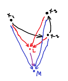
We define a cone to $\mathcal{C}$ as an object $M$ together with morphisms $m_i:M\to X_i$ such that it commutes with the existing diagram (formally, such that for every morphism $f:i\to j$ in $\mathcal{I}$, we have $F(f)\circ m_i=m_j$).

Now this necessarily represents an object with "more information than each $X_i$" -- so we're interested in the "infimum" of these cones, the one with the least information, the one to which there exists a morphism from any other cone. The limsup of cones, if you will:

We define the limit $(L,\ell_i)$ of the diagram to be a cone such that for any cone $(M,m_i)$ to the diagram, $\exists!\ u:M\to L$ such that the diagram commutes, i.e. $m_i=\ell_i\circ u$ forall $i$.

The above diagram commutes, and the purple morphism is unique.

And the dual notion is also observed, a liminf:

We define a co-cone from $\mathcal{C}$ as an object $\overline{M}$ together with morphisms $\overline{m}_i:X_i\to \overline{M}$ such that it commutes with the existing diagram (formally, such that for every morphism $f:i\to j$ in $\mathcal{I}$, we have $\overline{m}_j\circ F(f)=\overline{m}_i$).

We define the co-limit $(\overline{L},\overline{\ell}_i)$ of the diagram to be a cone such that for any cone $(\overline{M},\overline{m}_i)$ to the diagram, $\exists!\ u:\overline{L}\to \overline{M}$ such that the diagram commutes, i.e. $\overline{m}_i=u\circ\overline{\ell}_i$ forall $i$.

The below diagram commutes, and the purple morphism is unique.

Alternatively, the limit and colimit may be characterised as the final object in the category of cones and the initial object in the category of co-cones respectively (check that this makes sense).

Examples:
Diagrams captioned by their limits.

	(empty diagram) Limit: final object Co-limit: initial object
	(discrete diagram) Limit: product Co-limit: co-product This answers the difficult cases of the empty product (it's just the final object) and the power (use the constant functor).
	(parallel diagram) Limit: equaliser Co-limit: co-equaliser

Exercises: Do some examples to convince yourself of the following ideas:

• Even if there are a bunch of morphisms in the diagram, the limit of the diagram talks fundamentally about the product of the "starting" objects of the diagram (think of: $X\rightarrow Y\leftarrow Z$, etc.).
• If your original diagram has non-commuting features, the limit of the diagram talks about equalisers of these features (think of: parallel diagram, reverse-parallel diagram $\leftrightharpoons$, other cycles, a diagram with non-trivial automorphisms).
• Adding commuting stuff doesn't change the limit (i.e. the limit of $X\to Y\to Z$ is the same if you add another morphism $X\to Z$).

---

Universal objects and comma categories

You may have noticed that images and coimages cannot be written as limits and colimits (do you see why?). We made a fairly specific specialisation when defining limits/colimits that doesn't really have to do with our "limsup/liminf" intuition -- we insisted we had morphisms either from or to the diagram, whereas we could in general have a more complicated property.

In general, instead of dealing with the category of cones, we could deal with some other category (called the comma category) and discuss its initial and final objects instead.

The key insight regarding this generalisation is as follows: one can see the limit as a construction in the category $\mathcal{C}^{\mathcal{I}}$ of diagrams in $\mathcal{C}$ of a certain shape $\mathcal{I}$. The limit object (which is an object in $\mathcal{C}$) can be "upgraded" to that category as the constant diagram (an element of $\mathcal{C}^{\mathcal{I}}$ that maps every node in the diagram shape to the same object in $\mathcal{I}$) (this "upgrading" is called the diagonal functor $\Delta: \mathcal{C}\to\mathcal{C}^\mathcal{I}:=\lambda M.\ (\lambda i.\ M)$) with a morphism to the object of $\mathcal{C}^\mathcal{I}$ we're actually taking the limit of.

So more generally, we can consider some category other than $\mathcal{C}^\mathcal{I}$, and a more general functor than $\Delta$, in order to formalise a more general notion of being a limiting object. We make the following definition:

We define the final morphism from a functor $F:\mathcal{C}\to\mathcal{D}$ to an object $D\in\mathcal{D}$ as a morphism $\ell:F(L)\to D$ such that for any morphism $m:F(M)\to D$, there $\exists!\ u: M\to L$ such that the diagram commutes, i.e. $m=\ell\circ F(u)$.

You may observe that $F$ generalised $\Delta$, $\mathcal{D}$ is the generalisation of the "category of diagrams", and the final morphism generalises the limit (with $L$ being the limit "object" in $\mathcal{C}$). Analogously we define, generalising the colimit:

We define the initial morphism to a functor $F:\mathcal{C}\to\mathcal{D}$ from an object $D\in\mathcal{D}$ as a morphism $\overline{\ell}:D\to F(\overline{L})$ such that for any morphism $\overline{m}:D\to F(\overline{M})$, there $\exists!\ u: \overline{L}\to \overline{M}$ such that the diagram commutes, i.e. $\overline{m}=F(u)\circ\overline{\ell}$.

These terms "final morphism" and "initial morphism" are not to be confused with the morphisms to and from an initial object or a final object, that we defined previously. Typically, these terms are used in neither context -- one simply says "universal morphism" to/from $D$ from/to $F$; and in the previous context, one simply says morphisms to a final object/from an initial object.

In general, these morphisms are referred to as universal morphisms or universal objects.

(By the way: the term "universal property" is just used to refer to the property of being initial or terminal or whatever.)

This notion can easily be restated as follows: given an object $D\in\mathcal{D}$ and a functor $F:\mathcal{C}\to\mathcal{D}$, one can construct the following:

The comma category $[F\to D]$ is a category whose objects are the morphisms $m:F(M)\to D$, and whose morphisms from $m_1\to m_2$ are given by morphisms $u:M_1\to M_2$ such that the diagram commutes, i.e. such that $m_1=m_2 \circ F(u)$.

The cocomma category $[D\to F]$ is a category whose objects are the morphisms $m:D\to F(M)$ and whose morphisms from $m_1\to m_2$ are given by morphisms $u:M_1\to M_2$ such that the diagram commutes, i.e. such that $m_2=F(u)\circ m_1$

Then a final morphism is the final object in the comma category, and an initial morphism is the initial morphism is the initial object in the cocomma category. If $\mathcal{D}=\mathcal{C}^{\mathcal{I}}$ (i.e. is a diagram category) and $F$ is the diagonal functor, then the comma category is the category of cones, and the cocomma category is the category of cocones.

One might dislike the asymmetry between $F$ and $D$ and decide to go a step further, generalising $D$ to another functor. So given two functors $F:\mathcal{A}\to\mathcal{D}$ and $G:\mathcal{B}\to\mathcal{D}$, we can construct:

The comma category $[F\to G]$ is a category whose objects are the morphisms $m:F(M)\to G(N)$ and whose morphisms from $m_1\to m_2$ are given by morphisms $u:M_1\to M_2,\ v: N_1\to N_2$ such that the following diagram commutes:

The previous definition of comma and cocomma categories then occur when $\mathcal{B}$ and $\mathcal{A}$ respectively are replaced by a singleton (and $D$ is the only object in their image in $\mathcal{D}$).

---

Examples: free group, image

Abstracting some categorical definitions

Before making any interesting definitions, we need to get something over with: the notions of injective and surjective homomorphisms do not really generalise very nicely to category theory -- the closest definitions are:

A morphism $f:X\to Y$ is a monomorphism if for distinct morphisms $g$ to $X$, $f\circ g$ are distinct.

A morphism $f:X\to Y$ is an epimorphism if for distinct morphisms $g$ from $Y$, $g\circ f$ are distinct.

One may check that all injective homomorphisms are monomorphisms and that all surjective homomorphisms are epimorphisms -- but it's not too hard to see that they are not equivalent. Concrete counter-examples exist even in simple categories like abelian groups.

If anyone has any motivation or insightful explanation of monomorphisms and epimorphisms, let me know. For example, are the non-injective monomorphisms (e.g. the quotient map $\mathbb{Q}\to\mathbb{Q}/\mathbb{Z}$) actually interesting or just something we need to get used to?

There are also related notions:

A morphism $f:X\to Y$ is a section if it has a left-inverse ("retraction"), i.e. a morphism $g:Y\to X$ such that $g\circ f=1_X$.

A morphism $f:X\to Y$ is a retraction if it has a right-inverse ("section"), i.e. a morphism $g:Y\to X$ such that $f\circ g=1_Y$.

It's clear that all sections are injective morphisms (and thus monomorphisms), and all retractions are surjective morphisms (and thus epimorphisms). Of course, these intermediaries are not category-theoretic.

One may define an isomorphism, denoted $f:X\leftrightarrow Y$, as a morphism that is both a section and a retraction. Here are some theorems about it:

An isomorphism has a two-sided inverse morphism.
Given $g_1\circ f=1_X$, $f\circ g_2=1_Y$ -- by considering $g_1\circ f\circ g_2$, we see that $g_1=g_2$.

A morphism that is both a monomorphism and a retraction is an isomorphism.
Since $f$ is a retraction, $f \circ g = {1_Y}$ -- so $f \circ g \circ f = f$. Left-cancelling (since $f$ is a monomorphism), $g\circ f = 1_Y$, thus $f$ is a section.

A morphism that is both a section and a epimorphism is an isomorphism.
Analogous to above.

---

Subobjects

In our minds, a sub-object is a subset that also carries the structure of that category -- in other words, it's isomorphic to another object in that category.

It's natural to identify the subobjects of $X$ then with injections (or rather monomorphisms) into $X$ (not with the domains of the injections, as they may have multiple embeddings into $X$). But the identification is not one-to-one -- multiple injections may have the same image. In general, two monomorphisms $g_1:S_1\hookrightarrow X$, $g_2:S_2\hookrightarrow X$ having the same image is an equivalence relation, expressible as:

$$\exists i:S_1\leftrightarrow S_2,\ g_1=g_2\circ i$$

So we identify the equivalence classes of monomorphisms into an object with its subobjects.

An alternate motivation for our definition of a subobject comes from the subspace topology (and vice versa), which is defined in terms of continuous inclusion maps. Of course, in our definition here, we allow the subspace topology to be any topology that allows an injective continuous map to the space, but the standard definition in topology asks for the coarsest such topology (i.e. the "least continuous" such map). Later, we will study some refined definitions of a lot of ideas here that may apply better to specific categories.

---

Quotient objects

The natural way to think of quotient objects in category theory is in terms of the first isomorphism theorem, which states that the quotient objects are the images of surjections from the object -- kinda "dual" to how subobjects are the images of injections into the object (keep this notion of "duality" in mind).

You might be afraid that this kind of defeats the point, since we'd like to eventually prove the First Isomorphism Theorem in category theory. Well, we'll do so with some other more category-specific definition of quotients, etc. so the First Isomorphism Theorem would simply be a demonstration that these two definitions are equivalent.

But once again, just identifying the quotient objects with epimorphisms overcounts them -- a single quotient can map to multiple different isomorphic things. So, as before, we write down an equivalence relation between epimorphisms from $X$: two epimorphisms $g_1:X\twoheadrightarrow Q_1$, $g_2:X\twoheadrightarrow Q_2$ are equivalent if:
$$\exists i: Q_1\leftrightarrow Q_2,\ g_2=i\circ g_1$$
So we identify these equivalence classes of epimorphisms as the quotient objects of an object $X$.

---

Products

One can take inspiration from the product topology, and think of the product of some objects as the object with the "least information" that still allows morphisms to each object. So we define:

Given a collection $X_i$ of objects, we define their product $\prod X_i$ as a collection of morphisms $\pi_i:X\to X_i$ such that:

1. For any other collection of morphisms $\pi'_i:X'\to X_i$, $\exists! u: X' \to X$ such that $\pi'_i=\pi_i\circ u$.

Question: what does the empty product look like? This definition seems a bit bad for this purpose. We'll develop some more general machinery in the next article or so.

---

Sums (aka "coproducts")

Shockingly enough, the "opposite" or "dual" of the above. Direct sums of vector spaces can be seen as the "smallest possible" (i.e. embedding into most possible things, i.e. having most possible information) vector space permitting morphisms from each vector space. Another example would be the disjoint union of sets. Perhaps this is even clearer with the free product of groups, where the free product is the object with the "most information possible" arising from your groups.

Given a collection $X_i$ of objects, we define their sum $\coprod X_i$ as a collection of morphisms $\varpi_i:X_i\to X$ such that:

1. For any other collection of morphisms $\varpi'_i:X_i\to X'$, $\exists! u: X \to X'$ such that $\varpi'_i=u\circ \varpi_i$.

Because of its "dual" appearance to the product (which we will soon see described more generally), the sum is often known as the "coproduct".

---

We'll now start to list subobjects and quotient objects related to a morphism. Here's a convenient cheat-sheet: the following diagram is commutative. (dotted lines are zero morphisms, which we will define shortly)

(play with it!)

---

Images

Next, let's think about the image of a morphism $f$. Once again, we can identify an image with a monomorphism, so we're really looking for a subobject consisting of monomorphisms $g$ with the same image as $f$. So we want an $e:I\to Y$ such that there exists a morphism $f_I: X\to S$ with $f=e\circ f_I$ -- but this is not enough, $I$ may be "too big" (it may contain elements that map to $Y$ not in the image), so we define:

A monomorphism $e:I\hookrightarrow Y$ is the image of a function $f:X\to Y$ if:

1. $\exists f_I:X\to I, f=e\circ f_I$
2. For any $e':I'\to Y$ and $f_{I'}:X\to I'$ such that $f=e'\circ f_{I'}$, there $\exists! u:I\to I', e=e'\circ u$.

This relies on the following key lemma of course: the images of $f$ form a subobject. This follows straightforwardly from the second condition.

---

Zero objects

Many categories have the notion of a zero element in an object -- groups have identities, vector spaces have zero vectors, and let's not talk about rings and fields. And some, like topological spaces, don't.

But we can't talk about elements of an object in category theory. But perhaps the examples above give you an idea -- we have seen trivial groups and trivial vector spaces. Objects comprising only of the zero element -- let's call them zero objects. So maybe we can talk about the images of morphisms from these trivial objects to other objects, and they would represent zero elements.

The idea behind a zero element is that it is "privileged" in some sense -- a morphism must preserve it. Furthermore, every object contains a zero element, so there must always be morphism from the zero object to any object. These criteria fixes a unique morphism from the zero object to any given object. In fact, this idea is captured by the following definition.

A universal object or initial object $I$ is an object such that for any object $X$ in the category, there is a unique morphism $I\to X$.

But there is also another idea behind the notion of a zero object, that it carries the "minimum information" compatible with the category's structure. Recall our interpretation of a morphism as something that either retains or discards information -- mapping an object to a zero object means discarding "as much information as possible".

A final object $F$ is an object such that for any object $X$ in the category, there is a unique morphism $X\to I$.

Finally, a zero object is defined as an object that is both initial and final.

Perhaps a bit surprising at first (but trivially easily), but we can in fact see that the initial and final objects are respectively unique up to (unique) isomorphism -- just consider the unique morphisms between the two objects. The reason it's kinda incredible that we can do this in full generality, is that e.g. we can immediately see that the trivial ring is not an initial object (because the ring of integers is), because it can't be mapped to anything, something that seems like a technicality at first glance arising from the fact that 1 must be preserved by ring homomorphisms.

But if you think about it, the category theoretic argument also comes from the same fact -- it comes from the fact that you can't map the ring of integers to its own zero element, because that doesn't preserve 1. But if you didn't mandate that ring homomorphisms preserve the multiplicative identity, then the ring of integers would no longer be an initial object.

---

Zero morphisms, kernels and equalizers

When defining a kernel of $f:X\to Y$, we're looking for a subobject of $X$ that maps to the zero element in $Y$. Since in category theory, a subobject is an injection (from an object we'd typically view as isomorphic to the subobject), we're looking for a monomorphism (subobject) $k$ that composes with $f$ to give us a morphism that maps everything to the zero element, whatever that means.

OK -- so what does it mean? What's a morphism that maps everything to the zero element? Recall that we're thinking of the "zero element" as the image of a morphism from the zero object (which really means we're identifying it with a subobject, i.e. an equivalence class of monomorphisms). So we can associate with our desired morphism $o:X\to Y$ the morphism from $X$ to the zero object, which then embeds into $Y$ -- so we define the zero morphism as their composition:
$$o:=X\to O\to Y$$
Where $O$ is the zero object.
$$\dots$$
There is an alternate, more general definition of a zero morphism for categories without a zero object that nonetheless caputres the notion of a zero element.

Here's an alternate way to think about morphisms from and to a zero object. An initial morphism is essentially the "least surjective homomorphism possible". A final morphism is essentially the "least injective homomorphism possible". These are in line with our understanding of the zero object as the "smallest possible" object, or the one that contains the least information.

In line with the way we've thought of injectivity and surjectivity when defining monomorphisms and epimorphisms, we make the following definitions.

A morphism $f:X\to Y$ is an initial morphism (or right-zero morphism, or coconstant morphism) if for any $g,h: Y\to V$, $g\circ f = h \circ f$.

A morphism $f:X\to Y$ is an final morphism (or left-zero morphism, or constant morphism) if for any $g,h: W\to X$, $f\circ g = f\circ h$.

(Exercise: Check that the morphism from an initial object and the morphism to a final object satisfy this property.)

Further, one may observe that for $l:X\to Y$ final and $r:Y\to Z$ initial, $r\circ l$ is both an initial and a final morphism. So the right general notion of a "morphism that maps everything to the zero element" is a "a morphism that is both initial and final", or a zero morphism.

$$\dots$$
Anyway, we're obviously interested in monomorphisms $k$ to $X$ such that $f\circ k=o$. But these don't all represent the kernel -- they could represent subobjects smaller than the kernel. So we define the kernel as follows:

A monomorphism $k:K\hookrightarrow X$ is the kernel of $f:X\to Y$ if

1. $f\circ k=o_{KY}$
2. For any $k':K'\hookrightarrow X$ such that $f\circ k'=o_{K'Y}$, $\exists! u:K'\to K, k\circ u = k'$.

More generally:

Given morphisms $f_i:X\to Y$, their equaliser is a monomorphism $k:X\hookrightarrow X$ such that:

1. $f_i\circ k$ are equal for all $i$.
2. For any $k':K'\hookrightarrow X$ such that $f_i\circ k'$ are equal for all $i$, $\exists! u:K'\to K, k\circ u = k'$.

The kernel can then be understood as the equaliser of a morphism with the zero morphism.

Of course, these definitions lie on a key lemma: the kernel/equaliser is a subobject -- i.e. that for two kernels $k_1:K_1\to X$ and $k_2:K_2\to X$, there $\exists i:K_1\leftrightarrow K_2, k_1=k_2\circ i$ -- this follows straightforwardly from the second condition in the definition.

---

Cokernels, coimages and quotienting by a subobject

I once said that one of the points of learning linear algebra was as an introduction to ideas that appear repeatedly throughout algebra. Here's where we really see this in action.

Recall the notion of a left null space $\mathrm{ker}(f^T)$ from linear algebra -- it sort-of represented the "space of constraints" on the image of a morphism, in that it was the orthogonal complement of the image $\mathrm{im}(f)$ in the co-domain. It represents the stuff that the image can't fall into -- or tying back into our understanding of morphisms as things that "cannot create information that wasn't already present in the domain", it represents the information the morphism hasn't created (whether or not it could have), a measure of non-surjectivity.

Well, "orthogonal complement of the image" is not something restricted to vector spaces -- we can understand it more generally, as a quotient. Interestingly, it would then no longer be a subobject, which I suppose is reasonable -- we don't really have a notion right now of what a transpose morphism is in a general category.

In general, though, the quotient we're looking for is not $Y/\mathrm{im}(f)$ -- clearly, that wouldn't exist in a lot of important categories, e.g. groups. That's only true in categories that seem "abelian" in some sense. Perhaps this is unsurprising, because we're thinking of the cokernel as "the information that the morphism has not created", and information is more than just elements of the set.

So the appropriate way to generalise "a quotient by the image" is to look at a quotient object of the codomain $Y$ (which, recall, is an epimorphism from $Y$) that composes with $f$ to produce the zero morphism. But dually in the case of the kernel, we must make sure that our quotient is the full, "most universal" one:

Given a function $f:X\to Y$, we define its cokernel as an epimorphism $\bar{k}:Y\to\bar{K}$ such that:

1. $\bar{k}\circ f = o_{X\bar{K}}$
2. For any other $k':Y\to\bar{K}'$, there $\exists! u:\bar{K}\hookrightarrow\bar{K}'$ such that $k'=u\circ k$.

Once again, the latter property shows that the equivalence class of these epimorphisms is indeed a quotient object.

In fact, this "composition forms the zero morphism" notion is the generalisation of the "quotient by an object" notion, or of the so-called exact sequence below. Generally, given a subobject $S$ given by some monomorphisms $s:S\to X$, the epimorphisms $q:X\to Q$ that always compose with these monomorphisms to form the zero morphism $q\circ s = o_{SQ}$ define the quotient $X/S$, if they are a quotient object.

$$O \to \ker f \to X \overset f \longrightarrow Y \to \operatorname{coker} f \to O$$
Oh, and an exact sequence is exactly the idea behind quotienting by an object.

$$\dots$$
Now recall the notion of a row space $\mathrm{im}(f^T)$. Once again, the row space is best interpreted as a quotient object of $X$ (in the case of linear algebra, the quotient by $\mathrm{ker}(f)$). But constructing it in terms of the kernel would clearly be quite complicated -- and perhaps not generally so useful. A better, more "general" approach is to think of an element of the row space as an equivalence class of elements that are mapped to the same element. So we define:

Given a function $f:X\to Y$, we define its coimage as an epimorphism $\bar{e}:X\twoheadrightarrow \bar{I}$ such that:

1. $\exists f_{\bar{I}}:\bar{I}\to Y, f = f_{\bar{I}}\circ \bar{e}$
2. For any other epimorphism $\bar{e}':X\twoheadrightarrow \bar{I}'$ and $f_{\bar I'}:\bar{I}'\to Y$ such that $f = f_{\bar I'}\circ \bar{e}'$, there $\exists! u: \bar{I}'\to\bar{I}, \bar{e}=u\circ \bar{e}'$

Which is again clearly a quotient object.