Bayes, bias, p-hacking and the Monty Hall problem

TL;DR: Bias is a fundamental concept in the science of agents; bias of a source is fundamentally related to cognitive bias.

---

You open the news in the morning, and you see the following headline from The Pan-Pan times: 80% of Chimpanzee Party lawmakers have criminal cases filed against them.

"Outrageous!" You cry-- "The Chimpanzee Party has no respect for the law! I certainly shall not be voting for them!" 

But upon subsequent investigation, you find that while this statement is true, in fact, 80% of Bonobo Party lawmakers also have criminal cases filed against them. Or perhaps you find that they have criminal cases filed against them -- in an unrecognized country created by some crackpot on Reddit. And the person responsible for generating these headlines was aware of this fact.

You feel cheated, even though everything you heard was the truth. Even though The Pan-Pan times only gave you information, and you acted as a rational agent when exposed to this information (well, actually you didn't, but let's ignore that for now), you feel like you've been "exploited" somehow, "tricked" even. 

Is this truly possible? Can a Bayes-rational agent truly be fooled by cleverly selecting information to provide?

Let's think about the problem more carefully. 

Our ultimate decision might be governed by the following rule: vote for whichever party you expect to have fewer criminal cases filed against its lawmakers. We may have some prior distribution on the fraction of criminal-accused lawmakers of each party, say $\mathrm{B}(2,3)$ and $\mathrm{B}(3,2)$ for the Chimpanzee and Bonobo parties respectively. Under the prior, the expected fraction of criminal-accused lawmakers are 0.4 and 0.6 respectively, and one would vote for the Chimpanzee Party; under the posterior, the expected fraction of criminal-accused lawmakers are 0.8 and 0.6 respectively, and one would vote for the Bonobo Party. 

Or.

Our ultimate decision might be governed by the following rule: vote for whichever party minimizes the expected sum $X_1+\dots+X_{100}$, where say: $X_1$ is the regulatory burden the party will place upon coming to power, $X_2$ is the tax rate the party will implement upon coming to power, $X_3$ is the number of criminal cases against the party lamakers, $X_4$ is the number of bad words the party's candidates use on TV, $X_5$ is the number of lies the party's candidates say on TV, $X_6$ is the number of dissidents the party will throw in prison upon coming to power, etc.

Let's say, for simplicity, that these are all Bernoulli distributed variables -- further that each $X_i$ (Chimpanzee Party) and $Y_i$ (Bonobo Party) are distributed as $\mathrm{Bernoulli}(0.5)$. Then in this prior distribution, we would be uncertain as to whom to vote for, as both parties have $\mathrm{E}[\sum X_i]=50$ is lower. 

And suppose the Pan-Pan Times tells us: "We looked at $X_{3}$ and it turned out to be 1 for the Chimpanzee Party!" Now, $\mathrm{E}[\sum X_i]=50.5$, while $\mathrm{E}[\sum Y_i]=50$, so we vote for the Bonobo Party. 

But here's the thing though: the precise information you receive isn't $X_3$ is equal to 1 -- it is the Pan-Pan Times's report is "$X_3$ is equal to 1". And that's what you should be conditioning on.

If you were to condition on the Pan-Pan Times's report is "$X_3$ is equal to 1" (call this variable $\Pi$), well, what would your inference look like? You could apply Bayes's theorem, etc. but simply put -- let's say the Pan-Pan Times's report is some generative process that looks at all the $X_i$, and reports one that is equal to 1 (i.e. tosses a hundred coins and reports a heads) -- it can do so in all but $2^{-100}$ of outcomes, so the only information we're given is that that particular outcome (where all $X_i$ are 0) is not the case -- the only information we're given is that the Chimpanzee Party isn't literally perfect -- so that $\mathrm{E}[\sum X_i] = 50/(1-2^{-100})$.

(OK, in this case, the decision is the same -- but for example, suppose our decision was instead "donate some sum of money proportional to the difference in $\mathrm{E}[\sum X_i]-\mathrm{E}[\sum Y_i]$" then the decision would be different.)

To instead condition on just $X_3=1$ -- rather than the full information provided -- is a cognitive bias. As actually implementing Bayes's theorem everywhere is expensive, the mind processes information using heuristics -- one such heuristic is that only some information is selected to be conditioned on, leading to selection bias. Indeed, all such "source biases" are fundamentally manifested as some form of cognitive bias -- the use of negative terms to describe the Chimpanzee Party, for example, is the exploitation of some sort of the association fallacy, repeating the word "Bonobo Party" for hours on screentime is an exploitation of the availability heuristic, etc. 

A perfectly Bayes-rational agent -- that takes into account all information it is exposed to -- is immune to being tricked in this way. But a real agent, which uses heuristics, can be exploited. The idea is that if such biases are systematic, then it can be predicted and avoided cheaply. 

Information theory of multiple random variables

In the previous articles [1] [2] we defined the information of an observation as the logarithm of its probability -- and its entropy of a random variable as the expected amount of information gained from observing it (and thus is a measure of how little information the prior carries). Naturally in the multivariate case it is trivial to define a "joint information" that is the logarithm of the joint distribution. and we have the joint entropy:

$$H(\mathbf{X})=-\sum_{\mathbf{x}}{p(\mathbf{x})\log p(\mathbf{x})}$$

Because the full joint distribution is at least as informative as the marginal distributions taken separately, we have the property:

$$H(X,Y)\le H(X)+H(Y)$$

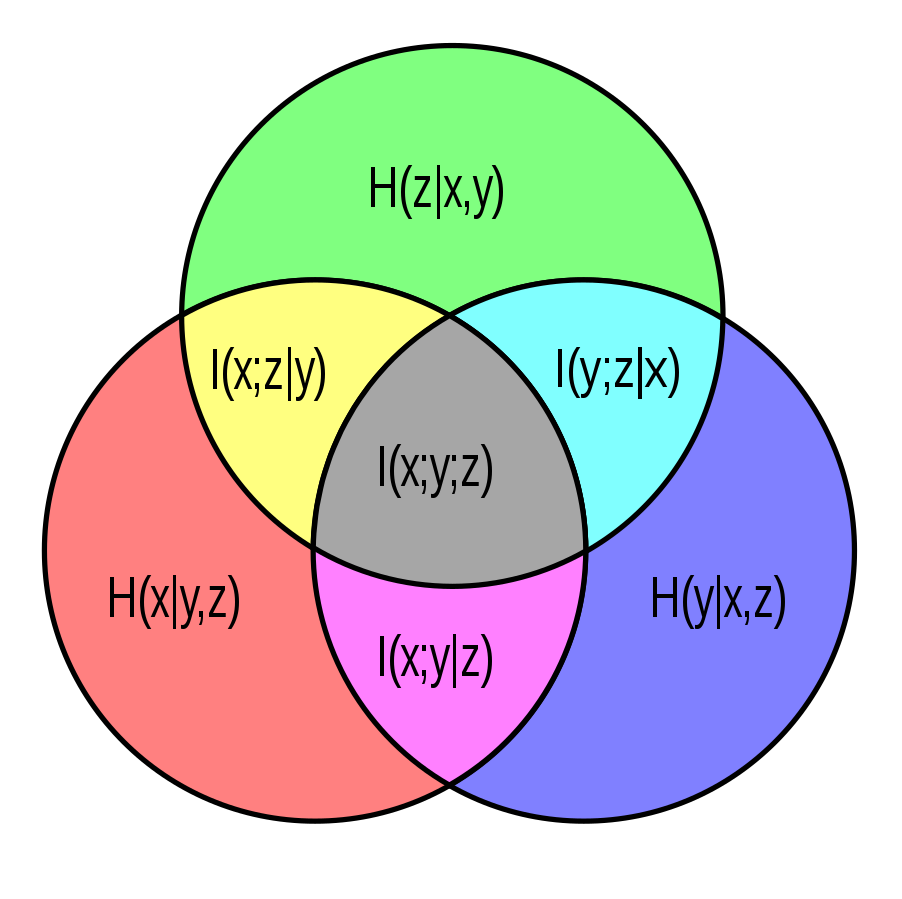
We often informally explain notions of independence and relationships between random variables in terms of information -- with information theory, we can now formalize these descriptions. The Venn diagram below shows the additive relationships between various entropies of multiple random variables:

(source)

$H(X)$ and $H(Y)$ are represented by the respective circles, $H(X,Y)$ is represented by the combined area of the circles and the mutual entropy; conditional entropies are as indicated. The mutual entropy (more commonly mutual information) is the expectation of the mutual information (more commonly pointwise mutual information):

$$\operatorname{pmi}(x;y) \equiv \log\frac{p(x,y)}{p(x)p(y)} = \log\frac{p(x|y)}{p(x)} = \log\frac{p(y|x)}{p(y)}$$

Even though the pointwise mutual information may be positive or negative (the probability distribution of $y$ may become more or less uncertain depending on the observed $x$), its expectation is always positive in a way analogous to conservation of expected evidence. These ideas can be generalized to beyond two variables:

(source)

The mutual entropy represents the reduction in the number of bits necessary to encode two correlated variables together, as opposed to separately. This is a special example of the entropy gain (or "Kullback-Leibler divergence") of two probability distributions $p$ and $q$: it is the expected number of extra bits used when expressing a $p(x)$-distributed random variable with a $q(x)$-entropy encoding. The mutual entropy is the entropy gain from $f_{X,Y}(x,y)$ of $f_X(x)f_Y(y)$.

$$\begin{align*}KL(p(X) | q(X)) &= \sum-p(x) \log {q(x)} -  \sum -p(x) \log {p(x)} \\&= \sum p(x) \log \frac{p(x)}{q(x)}\end{align*}$$

The first term of this expression (the number of bits required to express the random variable in the incorrect encoding) is also known as the cross-entropy.

Frequentism as a bureacuratic restriction on speech

Although it is traditional to claim that Bayesian and frequentist statistics are two "schools" of probability and statistics, there are actually two distinct ideas that are labeled "frequentist" (and analogously "Bayesian"):

• Frequentist probability: An interpretation of probability, an alternative to the subjective interpretation of probability normally associated with Bayesianism. Under the frequentist interpretation, probability is understood as having to do with frequencies of observations, e.g. a probability of 1/2 means that you can expect 50 coin tosses out of 100 to come up heads. In reality, this merely shifts the problem to interpreting expectation instead of probability.
• Frequentist statistics: A formulation of statistical inference, in which we don't really discuss probabilities of theories at all, but restrict ourselves to talking about tautological statements about the probabilities of observations given theories. The supposed advantage of this is that we don't need to follow unproven beliefs about priors.

In the Bayesian view, the frequentist interpretation of probability appears as follows: given a random variable $X$, we sample a sequence of IID variables $X_i$ -- the "limiting" distribution of these $X_i$s is then seen as the probability distribution of $X$.

(From a "positivist"/"scientific" viewpoint, it is rather absurd to define the probability of heads on a coin-flip in terms of a large number of other coin flips. After all, it is only an approximate assumption that all these coin flips are distributed identically. The purest way to talk about IID variables would be to consider an infinite number of universes, each in which a coin flip occurs. Of course, if the universes were identical in every way, the coin flips would be the same in every universe and the probability of heads will be 0 or 1. Probability arises from the fact that we have limited information about the state of the universe -- thus the average is not being taken over all identical universes, but over all universes which match the limited information we have. This "purification" of frequentism is simply Bayesian probability, as the "set of universes" is just the sample space, and the distribution of the unknown information is a Bayesian prior.)

The reason that frequentist statistics is typically associated with frequentist probability is that frequentist probabilists see it as odd to talk about the frequency of a theory being true -- to them, the same theory is true in each experiment conducted, since frequentist probability does not consider the situations in "alternate universes". Of course, this distinction between theory and observation is completely arbitrary -- on a logical level, theories and observations are both just logical statements, and analogously parameters and observed quantities are both just random variables.

To "forbid" talking about the probability of a theory is simply a bureaucratic restriction on what one can say, not something that affects your decisions in any way. When it comes to making decisions, one has to compute expected utilities, which requires a Bayesian approach (because frequentism does not consider "multiple universes"). Even if you don't say the probability of a theory is 80%, and only say that the probability of some observation would be 95% given that theory, the fact that your discipline "accepts" a p-value of 0.05 itself implicitly means that you believe the theory to be true with sufficient certainty.

Positivism as the rejection of anthropic reasoning

The Sleeping Beauty problem

The following experiment is performed on Sleeping Beauty: on Sunday, she is put to sleep, after which a coin is flipped.

If the coin came up heads, she will be woken up once on Monday. If the coin came up tails, she will be woken up twice, on Monday and Tuesday.

Each time she is woken up (with no indication of given of what day/which instance it is), she is asked the odds that the coin came up heads, then her memory of the waking is wiped and she is put back to sleep.

Given that she knows how the experiment works, should she answer odds of 1/2 or 1/3?

The answer is obviously 1/2. That is the prior probability of the coin coming up heads, and being woken up gives her no new information -- it just tells her that she's been woken up at least once. She already knew she'd be woken up -- if she expects her odds at being woken up to be 1/3, then her odds would have already been 1/3 before she started the experiment (this is, of course, a standard trick).

$$P(H|W\ge 1)=\frac{P(W\ge 1|H)\cdot P(H)}{P(W\ge 1)}=P(H)=\frac12 $$
A very large number of people, however -- including on LessWrong -- argue that Beauty should answer "1/3", or that that "both answers are right, depending on how you formulate the problem", or something to that flavour.

But this is a perfectly well-posed problem -- both answers cannot be right. The LW post is right that I notice I am confused, but wrong about what I notice I am confused by.

I don't find the problem itself confusing. I find people's minds and people's intuitions confusing -- including my own, because I can certainly see the intuition for 1/3.

One might say that this is uninteresting -- it doesn't matter what you "feel", the truth is the truth.

Well, an important scientific skill is to correct your intuitions to reflect reality. When you learned about relativity, you had to fix your intuition about fixed lengths and time intervals by thinking about four-vectors. When you learned about quantum mechanics, you had to fix your intuition about there being an absolute reality by learning about state vectors and how observation projects it rather than revealing an underlying reality.

Because human heuristic reasoning/understanding/skip-aheads is almost entirely in terms of such mental models, i.e. intuition, I would go so far as to say that if you don't understand why your intuition goes wrong, you don't understand why it is wrong in the first place, because it is your intuition that reflects your understanding, your model of the physical world.

---

Fair bets

So why do you sometimes "feel" that the answer is 1/3, even when Bayes's theorem says it is 1/2?

I would explain my intuition in terms of Monte-Carlo simulations: I think -- "probability (kindasorta) means how many times will something be true if repeated, right?" So if we repeat the experiment 100 times, then out of the 150 times she's woken up, 50 times the answer would be "heads" and 100 times the answer would be "tails".

Or in other words, if Beauty had the option to bet which way the coin had come up (e.g. she gets 1pt if her prediction is correct, 0pt if wrong), then if she consistently bet tails, she'd end up with 100pt, while if she consistently bet heads, she'd end up with 50pt.

And what of her making this bet before the experiment begins? What if she is given a choice, before the experiment begins to either: (a) bet, when she wakes up, that the coin came up heads or (b) bet, when she wakes up, that the coin came up tails?

Aha! But that's not a fair bet! That's giving her the option to bet twice that the coin came up heads, or bet once that the coin came up tails -- which is really a bet offering her 2:1 odds on the coin coming up tails -- so of course she should take tails.

But that still doesn't eliminate our entire confusion. Sure, from the perspective of SleepingBeauty-before-the-experiment, this is a bet offering 2:1 odds ... but from the perspective of SleepingBeauty-who-just-woke-up, there's no 2:1 odds, is there?

---

A prisoner's dilemma against a temporally-displaced copy of yourself that may or may not exist

When Beauty wakes up, she knows that there is a 1/2 probability that the coin came tails, and so a 1/2 probability that there will be another time she'll be woken up and asked the same question, offered the same bet -- and a 1/2 probability that that the coin came up heads, and so a 1/2 probability that there won't be such a time.

So she is really playing Prisoner's Dilemma against an identical copy of herself. If she chooses heads, then her twin -- who may or may not exist -- will also choose heads, because two identical copies cannot act differently. If she chooses tails, then that possibly-existent twin will also choose tails.

So if the coin came out heads (of which there's a 50% chance), then her choosing heads will lead to a payout of 1pt, but if the coin came out tails, then her choosing tails will lead to a payout of 2pt.

So if Beauty accepts evidential decision theory, she will, in fact, win, while also holding the true belief about the probability of a heads -- 1/2. Of course she will lose if she accepts causal decision theory, but that's fine -- causal decision theorists lose all the time.

(In fact there is a problem that even EDT seems to fail at, which I will discuss in a future post, but this has nothing to do with anthropics and Sleeping Beauties, so I don't believe it to be relevant here.)

---

Positivism vs. Anthropic reasoning

The "halfer" argument can be considered a rejection of anthropic reasoning. Anthropic reasoning can be illustrated with simpler, less unwieldy examples:

• Bostrom's Simulation Argument: If we are not living in a computer simulation, then it is unlikely that humans will ever make a large number of universe simulations, so we'll probably go extinct very soon or something. Also Boltzmann brains.
• Celibate Adam: You are the Bibilical Adam, and decide, on a whim, to procreate with Eve if and only if a coin toss comes up heads. So an anthropist Adam reasons that the coin toss will almost certainly come up tails, because what are the odds that he has billions of progeny and he just happened to be in this body?

The last riddle makes the problem with anthropic reasoning manifestly obvious, since the decision to only count human bodies and not animals, rocks, and random disparate sets of particles is a completely arbitrary one. 

Anthropic reasoning carries an underlying assumption that there is some metaphysical process that randomly allocates "souls" into human bodies. The basic belief of the anthropists is that metaphysical claims can be information -- like "I am conscious" (note that the basic problem here isn't "conscious" as much as it is "I").

Well, I obviously don't have much respect for this sort of fluff -- I simply reject this kind of thing at the level of epistemology.

The fundamental lesson of logical positivism is that your beliefs should not depend on your metaphysical gauge -- in particular, they should not depend on whether you believe in philosophical zombies (or rather, what you consider to be philosophical zombies), universal minds or many worlds.

The model of Celibate Adam problem according to anthropists.

And by the way, this also explains the "non-anthropic equivalents" that anthropists provide for anthropic problems -- these non-anthropic equivalents are just scenarios which make these metaphysical models real. For example, the "non-anthropic equivalent" of the Sleeping Beauty problem looks like this (and I encourage you to work it out before reading):

There are two Awake Beauties. A coin is flipped -- if the coin comes up Heads, then one Awake Beauty is randomly selected for interview; if the coin comes up Tails, then both Awake Beauties are interviewed. You, who are one of the Awake Beauties, are interviewed -- what is your credence for the coin having come up heads?

The model of Sleeping Beauty problem according to anthropists.

And these sorts of "metaphysical models" are implicit in the betting-based arguments -- when you say, "people in computer simulations would benefit from betting that they are, so so should you", you are in effect putting yourself in the same category as the simulated people to set up the frequentist "experiment". But whether what the simulated people should do is correlated with what you should do is entirely a matter of your Bayesian prior, and there's nothing in the prior that requires anthropic considerations.

By the way, this is why frequentism cannot be a fundamental basis of defining probability. E.g. if you're trying to place odds on an unfair coin toss, and you say "well, my coin-tosses have been 75-25 so far, so that means the probability is 75-25", then you are making the arbitrary decision that the results of your previous coin-tosses predict the next one, you are arbitrarily putting them in the same category. Your Bayesian prior is what justifies this categorization, this believed correlation, the belief that some weird systematic gust of wind won't affect your 101th toss, your Bayesian prior is what lets you do sample tests. Sample tests are not a definition of probability, and in the absence of sample tests -- i.e. without assuming known correlations between some observed phenomenon and the phenomenon you're trying to predict -- like in the case of questions like "what is the probability of us being in a simulation?", your prior is all that matters.

And so similarly with Doomsday arguments, "the mediocrity assumption" or "the Copernican assumption" is just some basically arbitrary Bayesian prior (and in that case we do have additional evidence that correlates with whether the world will end or not, so we should be updating this belief, in whatever direction, and mediocrity should not be the basis of our decisions, just like how we have information on human life expectancies, so a 5-year old should not believe that he will die at 10).

In the Sleeping Beauty problem, if you replaced the monetary reward for something completely short-term, like a cookie, so Beauty does not care about whether her other awakening gets it or not, then betting on tails no longer gives her an advantage over betting on heads. You might say "well, but if she always bets on tails, she gets twice as many cookies", but this is irrelevant -- there's no reason to regard that as a relevant frequentist experiment that affects her beliefs about the probability of the coin coming up heads. Her prior is 50-50, and no new (real, non-metaphysical) information has been introduced to her. 

Hacking Evidential Decision Theory

In the previous article, we discussed the Sleeping Beauty problem, rejected anthropic reasoning and and explained how the "halfer" position is the correct one and it only "loses" if you accept Causal Decision Theory, but that's okay since CDT agents lose all the time.

Well, upon some thinking, it seems that agents EDT agents can also lose, but this has nothing to do with anything anthropic. Here are two equivalent (to each other) problems that "beat" Evidential Decision Theory:

• Vincent Conitzer (2017) (simplified version):  Two coins are flipped. Our good friend and lab rat Sleeping Beauty is woken up on (if HH or HT) Monday and Tuesday (if TH) Monday and Wednesday (if TT) Tuesday and Wednesday. When woken up, she is told what day it is, and offered the following bet: "1pt for correctly guessing Heads, 3pt for correctly guessing Tails". Should she take the bet?

In terms of precommitment, committing to bet heads means an expected return of 1pt, while committing to bet tails means an expected return of 1.5pt. So she should bet tails.

But if she wakes up on Monday (or symmetrically Tuesday), then betting heads means an expected return of 1.33pt, while betting tails means an expected return of 1pt. So she bets heads.

(The problem can be formulated in terms of sending two different agents into rooms, so there's nothing anthropic/memory loss/splitting people in two about this.)

• Psy-Kosh's non-anthropic problem: You have 10 identical agents with shared finances. Flip a coin -- if Heads, send 9 agents to green rooms and 1 agent to a red room. If Tails, send 1 agent to a green room and 9 agents to red rooms. Offer the agents in green rooms $(G-3R)$pt, where $G$ and $R$ are the number of agents in green and red rooms -- and the offer is executed only if all agents agree to accept it. Should they take the offer?

If the coin comes up heads, $G-3R=6$. If the coin comes up tails $G-3R=-26$. 

In terms of precommitment, we know that the probability of heads is 50%, and the expected gain from taking the bet is -10pt, so the agent's shouldn't take the bet.

But when an agent actually wakes up in a green room, it figures that means a 90% chance of Heads, and the expected gain from taking the bet is 2.80pt.

I.e. you end up with maybe 1, maybe 9 green agents who think -- perfectly rationally -- "what are the odds of there being just one green agent and it happening to be me?" and assign 10% odds to that possibility, and therefore to Tails, even though 50% of the cases are actually Tails, because 90% of the times that you end up in Green, the coin has come up Heads. 

It seems that superrationality is not good enough. 

+related to simpson's paradox?

Two ways to understand overfitting (and don't peek!)

Assorted comments on overfitting

The very first time I was introduced to the notion of overfitting -- by three diagrams of regression curves on scatter plots labelled as you may guess -- I became very uncomfortable. I was probably eleven years old, and did not understand Bayesian statistics, did not realize that seeing 51 heads out of a hundred didn't imply that the coin genuinely had a heads rate of 0.51.

Or rather: I didn't realize that I did realize that. If you had made me bet on the number of heads that would come up in the next hundred flips, I would not provide odds that would indicate an honest belief of seeing 51 heads.

(Because deep down, I had a non-uniform prior.)

And the same principle applies to drawing regression curves. You may insist that your curve with all its squiggles is "unbiased" or give any one of the terms (one for every squiggle) used to describe non-Bayesian estimators, but ultimately -- that's not the curve you'll bet on. You know it's just far more likely that those squiggles are the result of noise which will not be the same (or knowably correlated) in the next sample, than for them to actually be a determining feature.

Yes, maybe the 79th coin toss will always be a tail because of a tiny AI hidden in the coin that counts, or maybe it was the result of factors that affected the 79th coin toss that you just didn't measure. While your data should affect your beliefs, they shouldn't completely overrule your priors.

And that's the key idea behind overfitting (and really the Bayesian notion of probability in general) -- how will your model, based on your data, of perform if you exposed it to data it hasn't yet seen. Because using it on data it hasn't seen is the point of your model -- that is your purpose in building it.

So overfitting occurs when a model learns features specific to your particular data set that don't generalize well. There are two ways this can occur:

• The training set is a biased sample: E.g. MNIST digits are all centered (but suppose you're testing on non-centered digits), or your medical database is all from a particular country. 
• There is noise: I mean, of course there's noise -- it's a statistical problem. Even if the world were deterministic, you still don't have all the information in the world. And you should avoid your model using this noise to make predictions, since noise is, by definition, unpredictable.

The first is a more tractable problem -- it can often be solved by data augmentation (if you have a very good picture of exactly how the data set is biased) or transfer learning (if there's a good chance the model is picking up on important features so you can just train it on the ones it missed). It's important to develop interesting transfer learning algorithms to solve this anyway, as the way humans learn often involves biased samples (e.g. personal experience) and reasoning capacity to unbias their knowledge. 

(Not that humans do always do this -- people often do form beliefs based on mere personal experience, but humans are capable of reasoning more clearly.)

The second is a problem that requires algorithmic solutions that hint our neural network towards Bayesian solutions. Solutions like "well, parameters are just a priori unlikely to be very large, so let's penalize that" (Lasso/Ridge regression), or more complicated (to explain in a simple Bayesian way) regularization algorithms like cross-validation and early stopping.

Another unclassified comment on overfitting: it's very easy to mistakenly "peek" at the test data. Simply in the act of saying "hey, this model works well on the test data, let's choose it" you are already performing a simple algorithm that checks several models and chooses them based on their performance on the test data -- i.e. you are kinda training the model on the test data, even if it is not seen in your code, just in your choice of hyperparameters.

That's why developing some kind of "theory" of hyperparameter optimization and regularization techniques is of importance, so you actually have a theoretical justification for picking your models. 

(Of course, this is hard. We've always been picking models, haven't we? For example when we decide to model something as belonging to a particular family of distributions so we only have to optimize in a 1-dimensional parameter space instead of the literal theory-space. In a sense, machine learning is the way to avoid modeling, due to the universal approximation theorem -- and the hope is that we can eventually make the priors as human-like as possible, which is the eventual goal of hyperparameter optimization and regularization algorithms.) 

Bayes theorem, estimators and the theory of Amazon ratings

If you've ever bought something on Amazon, or looked at player ratings on an online game, you've often had to weigh the average rating against the number of ratings. A higher average rating is surely a good thing, but would you really prefer one 5.0 rating to a hundred 4.5 ratings?

The way to think about a question like this is to ask: What are we trying to maximise, here? What is it that we're trying to achieve?

We're trying to maximise what our own rating would be -- or rather, the expected value of what our own rating would be.

So we should think of the rating as a random variable with some distribution, whose true mean (and not the sample mean) is what we seek to estimate. It was not immediately obvious that the problem would be a statistical one, but it is now.

So, why don't we just use the sample mean to estimate the true mean, and trust the "unreliable" 5.0 rating over the "reliable" 5.0 rating? Three reasons:

• Items usually don't have a true 5.0 rating, and just one rating is unlikely to change our opinion of this.
• We're not really trying to maximise the expected value, e.g. we may be concerned about risk (i.e. a greater variance in the distribution of the true value of the rating is itself a negative, because a true 1.0 rating may mean the application is dangerous or contains viruses)
• Having fewer ratings may itself be an indicator of lower quality, because it's less popular.

In any case: the keyword is "belief distribution". The first point points out that we have a prior belief distribution and each rating updates this belief distribution. The second point points out that we need an idea of what the entire posterior distribution looks like, rather than just a point estimate.

Well, obviously, the solution is Bayesian statistics (link to the main Bayes's theorem article). If you have a prior distribution on the true mean, and a likelihood function for the observations, you can compute the posterior distribution via Bayes's theorem.

Exercise: Compute, in the case of just two possible ratings (upvote and downvote/like and dislike) the "correct" rating (say, mode of posterior) given a uniform prior. Derive the so-called Laplace's rule of succession. 

The Dirichlet (also Beta) distribution

Here's a category of distributions we may often want: a distribution on the simplex.

I.e. a multivariate distribution on $n$ nonnegative numbers that add up to 1. This is something that we can definitely see using as prior distributions on parameters that can be interpreted as "probabilities" of something. One can see that this is important for the Categorical and Multinomial distributions, for instance: and in the case of two numbers (i.e. a univariate distribution, since it's on a line segment), for the Bernoulli and Binomial distributions.

Here's one such distribution family that may come to your mind: for $x_i$ in the simplex $\sum_i x_i = 1$,

$$f(x_1,\dots x_n\mid\theta_1,\dots\theta_n)\propto \prod_{i}{x_i}^{\theta_i}$$
By adjusting the values of the $\alpha$s, one can get suitable priors that represent our beliefs correctly. This is known as the Dirichlet distribution, and its univariate case $f(x|\theta_1,\theta_2)\propto x^{\theta_1}(1-x)^{\theta_2}$ is known as the Beta distribution.

In fact the parameters of said distributions are usually provided a bit differently, with $\alpha-1=\theta$.

Exercise: Prove that:

• The normalization constant is given by $\frac{\Gamma\left(\sum_i\alpha_i\right)}{\prod_i \Gamma(\alpha_i)}$
• The mean is given by $E(X_i)=\frac{\alpha_i}{\sum_i\alpha_i}$
• The Dirichlet distribution is the conjugate prior to the categorical/multinomial distribution. This is the key fact that makes the Beta/Dirichlet distribution important.

I don't believe p-hacking is a problem.

Or more precisely: I don't believe p-hacking is a fundamental mathematical or statistical issue, but rather an issue with the methods adopted by experimental researchers.

If you haven't heard of p-hacking, it's as follows: suppose you want to find predictors for cancer. You test 100 possible predictors each at p-value 5%. Now although the chance of a false positive on any given test is 5%, you're expected to get 5 false positives in the test. So you can "always" find a (fake) predictor for cancer just by surveying enough things.

Another way of putting it: even if your factors don't actually predict cancer, the probability distribution for the observed correlation for any one factor may look something like this.

So when you test for these factors, when the correlations you observe actually sample the above curve, you're faced with a question: do you believe the points that lie in the shaded region (beyond your significance level) actually reject the null hypothesis?

On one hand: they lie beyond your significance level. Individually, you need to reject those null hypotheses.

On the other hand, one can also think of a "mega-" null hypothesis as implying the above curve: since your points sample the curve, you need to accept the null hypothesis.

---

I believe the answer is to reject those null hypotheses, i.e. to not make any "corrections" for having tested multiple parameters.

Here are some explanations:

• An individual researcher "p-hacking" is fundamentally/mathematically no different from a large number of researchers investigating of various different parameters. Surely it makes no sense to argue that all positive results in the literature should be ignored, or that they should be evaluated at much stronger significance levels. 
• When you investigate a large number of parameters, the probability of a true positive is also higher (in a Bayesian sense). If your positives are more likely to be false than true when you're testing a hundred parameters, they were more likely to be false than true when testing one parameter too. Of course, you are much more likely to have false positives when testing more parameters, but that doesn't increase the chance that any given deduction is false, because there are more true positives, too. 
• Or in other words, the "mega-null hypothesis" probably isn't true. If the $\theta$ parameters are independent, then you'll probably have a large number of false null hypotheses. The "mega-null hypothesis" argument actually seems to assume zero probability of a true positive. 
• Equivalently: just apply Bayes's theorem/the fact that probability is commutative. (equivalent to the first point)

Also note how the Bonferroni correction has nothing to do with p-hacking: it applies to looking at probabilities/confidence levels of several hypotheses being true, not about one.

---

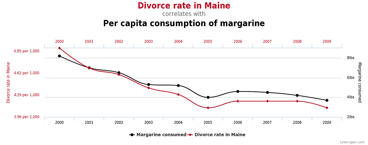
So, then, why do the consequences of p-hacking all seem to bizarre? Stuff like this:


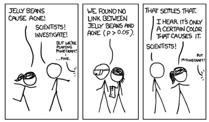
Or this:

Full comic for context: xkcd 882

Surely we don't actually believe that margarine causes divorces in Maine, or that only green jelly beans cause acne?

And no, we don't.

Why not?

Because there is no a priori reason to suspect that margarine causes divorces in Maine. Because a priori, we know that it's highly likely that whether green jelly beans cause acne is correlated with whether all the other color of jelly beans cause acne (because it's very unlikely that colour itself causes acne). These correlations should be embedded in our prior.

But these aren't fundamental issues with the nature of statistics. These are issues with how frequentist researchers may often decide which hypotheses to test. One should have some theoretical justification to formulate a hypothesis: that's how you know the prior probability is significant. Unless you have a good theoretical model for why a certain correlation/etc. should hold, the hypothesis should not be tested.

This problem is particularly prevalent in the social sciences, where a "general mathematical theory" of social science does not exist. Even in economics, you often end up with pseudo-science like this: Want to expand the economy? Tax the rich! (this particular study was terrible on several levels: (1) the conflation of correlation and causation -- this is always a problem when you have temporal trends, because time is a hidden parameter; that's why you should do cross-sectional studies (2) the correlation was statistically insignificant by any standard (3) there was no theoretical justification for why progressive taxation would expand the economy, leading to the problems discussed in this post.)

This point is essentially the point made by several papers (links: [1][2]) discussing "multiple comparisons in a Bayesian setting" -- it is what is meant by claims like "the multiple comparisons problem disappears when you use a hierarchial Bayesian model with correlations between your parameters".

Classical Statistics, Confidence Regions and Hypothesis tests

The basic general idea behind a confidence region is this: Given that the true value of some parameter is $\theta$ we may have some mechanism to sample "random regions" $R$ for $\theta$ such that 95% of these random regions contain $\theta$.

The first obvious issue is that this mechanism should not depend on $\theta$, as it is not known to us. We want a general experimental mechanism that for any $\theta$, produces random regions of the same confidence level ("95%").

In some basic cases, this is easy: for example, suppose we have some $X\sim N(\mu, 1)$. Then for any $\theta$, 95% of intervals generated as $X\pm 1.96$ contain $\mu$.

The key hint that you may find in the example above is that $\mu$ is a location parameter for $X$, i.e. the probability of $X\mid\mu$ is a function of just $X-\mu$, i.e. the distribution of $X-\mu$ itself does not depend on $\mu$, and is just $N(0,1)$. $X-\mu$ is what we call a pivotal quantity here.

In general, a pivotal quantity is a function of some data and the true value of the parameter itself $k(X,\theta)$ such that its distribution is completely specified. Then a confidence region for $k$ can hopefully be transformed back into a confidence region for $\theta$ at the same confidence level.

---

OK, next question: what is the implied prior of confidence region calculations? I.e. under what prior can the confidence level be interpreted as the probability that the true value of the parameter is contained in the confidence region?

(For a general prior, such a region that gives you some probability of containing the true value of the parameter is called a credible region.)

Well, what exactly is the confidence level? It's the probability that a randomly generated random region contains the true parameter value -- i.e. before you actually know what the random region is. Once you get the generated random region, this probability may change depend on the prior probability of the true parameter value being in this concrete region.

In other words, the implied prior is one such that $\theta$ has an equal prior probability of being in any possible confidence region. This is easy to calculate in some specific examples:

• If $\theta$ is a location parameter for $X$, the implied prior on $\theta$ is uniform, $\propto 1$.
• If $\theta$ is a scale parameter for $X$, the implied prior on $\theta$ is logarithmic, $\propto 1/\theta$.  

---

The way that hypothesis testing is first introduced, one talks of things like "the probability of finding a value of $x$ at least as extreme as you did". And one sometimes chooses a "one-sided" hypothesis test and other times a "two-sided" hypothesis test. It should be clear that this isn't too fundamental a concept to be interested in.

Rather, one sensible, more generally appropriate way of thinking of hypothesis tests is in terms of confidence regions. Specifically: testing a null hypothesis is equivalent to asking if it is contained within the confidence region of our data.

Obviously, this depends entirely on the shape we choose of our confidence region. We can always just choose a confidence region that includes or excludes our null hypothesis and maintain the same confidence level.

While it may be disappointing that there is no one way to construct a confidence region, this makes a great deal of sense. For example, consider the following multimodal distribution:

The sensible confidence region to construct would then be one that contains the bulk of both peaks. "Sensibility" in this sense is getting the confidence region of the least length (you may observe that this is not reparameterization-invariant).

Various different constructions of confidence regions is what gives you things like two-tailed and one-tailed tests.

Also read: Choosing the more likely hypothesis by Richard Startz

Machine learning as function approximation; statistical and cognitive motivations

The most general formulation of machine learning is that it is the attempt to approximate (or "learn") some mathematical object. For example:

• Regression attempts to approximate a function.
• Classification attempts to approximate an equivalence relation.
• Dimensionality reduction attempts to approximate a parameterization.
• Generative neural networks attempt to approximate a distribution (i.e. a sampler).
• Representation attempts to approximate a compression algorithm.
• Game-theoretic learning (e.g. reinforcement learning, no-regret learning) attempts to approximate a distribution of strategies. 
• Neural networks in NLP attempt to approximate a vector space that effectively represents desired relationships between words.

The Data Science course addresses several "toy algorithms" that discover low-order or simplified approximations. There are two -- different -- explanations of what more "AI-esque" machine learning is, which also lead to two different motivations for machine learning, and two different ways to understand each neural network architecture and each of some ideas in machine learning.

1. The statistical motivation -- machine learning is a non-linear generalisation of "linear" statistical techniques (data mining) like linear regression, PCA and linear decision boundaries. One can always do these linear techniques with some transformation of the data that makes relationships linear (while making sure the transformation is not absurd), but you need a way to "train" what the right such function is. In this sense, machine learning acts as a function approximator.
2. The cognitive science motivation -- a computer should be able to do whatever a brain can, but how exactly does a brain do the stuff it does? To take a simple example, the brain can recognise digits -- well, whatever the brain does, it takes an image as input and outputs a digit, i.e. it's a function. So once again, we need a function approximator.

Great. So machine learning is about making function (or object) approximators. The basic idea is that we're looking for a function that minimises the overall error for a population of data -- it's basically a calculus of variations problem, isn't it? Well, except it isn't, because we don't have access to the entire population, so we need to avoid overfitting (i.e. we need to consider a Bayesian prior). This is also what we meant by "making sure the transformation is not absurd" as we mentioned.

As a general rule, I'd say that if a feature of human brains are present at birth, we should expect to have to hard-code it, while if a feature is learned by humans, we should definitely get our AI to learn it, too (this is the "converse" of a general rule I have when trying to organize knowledge about biology in my head, which is we pretend that evolution is not an algorithm but a hard-coding, simply because actually trying to simulate an evolutionary algorithm in a highly complicated environment is hard). So for example, the transformations that a spatial transformer network finds acceptable are hard-coded, because we didn't actually need to stand on our head or squish our eyes with a truncheon to learn how to read squished-up text. 

Anyway, we want a universal function approximator -- a system that can generate a function arbitrarily close to any given function given sufficiently many parameters. A basic example of such a system is polynomial regression, but for most applications this has the wrong Bayesian prior (it gives zero prior probabilities to high-order polynomials, but most machine learning applications require functions with heavy non-local effects).

Another function approximator is a neural network. That a neural network (even of single layer) is a universal approximator is called the universal approximation theorem, i.e. functions can be written as linear combinations of some scaled and translated sigmoid functions.

(Exercise: explain why the universal approximation theorem is true for the sigmoid function. What other kinds of functions is it true for? It's actually not that hard at all. If you do get stuck, check out the visuals in Michael Nielson's e-book. A rigorous proof can be found here.)

In fact, the universal approximation theorem is not actually particularly important at all to the success of neural networks -- like we said, plenty of systems are universal approximators, but they don't have the right Bayesian prior (and this matters when you have limited data). The single-layer neural network actually has a bad implied prior for many tasks, which is why we usually study "deep" neural networks, which have a surprisingly good prior.

I have seen many explanations as to why this is so: deep learning means doing things in steps, deep learning corresponds to decomposing "hierarchy" or "structure" in the world and our world is "inherently hierarchial", etc. But honestly, these all seem like terrible rationalizations -- I don't even see how these claims are testable. You would need to create a system that isn't "inherently hierarchial" and demonstrate that deep learning doesn't do very well on it (which, as far as I can see, makes no sense). The right way to "explain why deep learning works so well" is to compute the implied prior and find out how it scales with depth.

Someone do this.