Showing posts with label statistics. Show all posts

Bayes, bias, p-hacking and the Monty Hall problem

TL;DR: Bias is a fundamental concept in the science of agents; bias of a source is fundamentally related to cognitive bias.


You open the news in the morning, and you see the following headline from The Pan-Pan times: 80% of Chimpanzee Party lawmakers have criminal cases filed against them.

"Outrageous!" You cry-- "The Chimpanzee Party has no respect for the law! I certainly shall not be voting for them!" 

But upon subsequent investigation, you find that while this statement is true, in fact, 80% of Bonobo Party lawmakers also have criminal cases filed against them. Or perhaps you find that they have criminal cases filed against them -- in an unrecognized country created by some crackpot on Reddit. And the person responsible for generating these headlines was aware of this fact.

You feel cheated, even though everything you heard was the truth. Even though The Pan-Pan times only gave you information, and you acted as a rational agent when exposed to this information (well, actually you didn't, but let's ignore that for now), you feel like you've been "exploited" somehow, "tricked" even. 

Is this truly possible? Can a Bayes-rational agent truly be fooled by cleverly selecting information to provide?

Let's think about the problem more carefully. 

Our ultimate decision might be governed by the following rule: vote for whichever party you expect to have fewer criminal cases filed against its lawmakers. We may have some prior distribution on the fraction of criminal-accused lawmakers of each party, say $\mathrm{B}(2,3)$ and $\mathrm{B}(3,2)$ for the Chimpanzee and Bonobo parties respectively. Under the prior, the expected fraction of criminal-accused lawmakers are 0.4 and 0.6 respectively, and one would vote for the Chimpanzee Party; under the posterior, the expected fraction of criminal-accused lawmakers are 0.8 and 0.6 respectively, and one would vote for the Bonobo Party. 

Or.

Our ultimate decision might be governed by the following rule: vote for whichever party minimizes the expected sum $X_1+\dots+X_{100}$, where say: $X_1$ is the regulatory burden the party will place upon coming to power, $X_2$ is the tax rate the party will implement upon coming to power, $X_3$ is the number of criminal cases against the party lamakers, $X_4$ is the number of bad words the party's candidates use on TV, $X_5$ is the number of lies the party's candidates say on TV, $X_6$ is the number of dissidents the party will throw in prison upon coming to power, etc.

Let's say, for simplicity, that these are all Bernoulli distributed variables -- further that each $X_i$ (Chimpanzee Party) and $Y_i$ (Bonobo Party) are distributed as $\mathrm{Bernoulli}(0.5)$. Then in this prior distribution, we would be uncertain as to whom to vote for, as both parties have $\mathrm{E}[\sum X_i]=50$ is lower. 

And suppose the Pan-Pan Times tells us: "We looked at $X_{3}$ and it turned out to be 1 for the Chimpanzee Party!" Now, $\mathrm{E}[\sum X_i]=50.5$, while $\mathrm{E}[\sum Y_i]=50$, so we vote for the Bonobo Party. 

But here's the thing though: the precise information you receive isn't $X_3$ is equal to 1 -- it is the Pan-Pan Times's report is "$X_3$ is equal to 1". And that's what you should be conditioning on.

If you were to condition on the Pan-Pan Times's report is "$X_3$ is equal to 1" (call this variable $\Pi$), well, what would your inference look like? You could apply Bayes's theorem, etc. but simply put -- let's say the Pan-Pan Times's report is some generative process that looks at all the $X_i$, and reports one that is equal to 1 (i.e. tosses a hundred coins and reports a heads) -- it can do so in all but $2^{-100}$ of outcomes, so the only information we're given is that that particular outcome (where all $X_i$ are 0) is not the case -- the only information we're given is that the Chimpanzee Party isn't literally perfect -- so that $\mathrm{E}[\sum X_i] = 50/(1-2^{-100})$.

(OK, in this case, the decision is the same -- but for example, suppose our decision was instead "donate some sum of money proportional to the difference in $\mathrm{E}[\sum X_i]-\mathrm{E}[\sum Y_i]$" then the decision would be different.)

To instead condition on just $X_3=1$ -- rather than the full information provided -- is a cognitive bias. As actually implementing Bayes's theorem everywhere is expensive, the mind processes information using heuristics -- one such heuristic is that only some information is selected to be conditioned on, leading to selection bias. Indeed, all such "source biases" are fundamentally manifested as some form of cognitive bias -- the use of negative terms to describe the Chimpanzee Party, for example, is the exploitation of some sort of the association fallacy, repeating the word "Bonobo Party" for hours on screentime is an exploitation of the availability heuristic, etc. 

A perfectly Bayes-rational agent -- that takes into account all information it is exposed to -- is immune to being tricked in this way. But a real agent, which uses heuristics, can be exploited. The idea is that if such biases are systematic, then it can be predicted and avoided cheaply. 

Machine learning and information theory

A simple and abstract way to look at machine learning is as a method to find optimal data compression algorithms (and indeed, data compression can be used as a measure of general intelligence). Fundamentally, the following two goals are equivalent: (1) approximating the distribution of some data (2) finding the optimal representation (compression algorithm) for said data -- the optimal representation is just the entropy encoding given the distribution.

Note that all of this is said about unsupervised learning algorithms -- generative modelling, dimensionality reduction/clustering, etc. -- but such structure in the data can also be uncovered during supervised learning (e.g. decision trees can emulate hierarchical clustering, feed-forward neural networks embed data into its feature representations), when the desired labels depend strongly on the clustering.

In supervised learning, you are no longer seeking to simply find an optimal compression for the data, but a compression that "agrees" with the labelling -- you are no longer seeking a representation that best predicts the original data, but a representation that best predicts the labels. In other words, in unsupervised learning you are trying to find a representation of fixed length $T(X)$ that maximizes the expected information that a representation provides on the data, the mutual entropy $I(X;T(X))$; in supervised learning you are trying to find a representation $T(X)$ that maximizes the expected information that a representation provides on the labels $I(y;T(X))$. This is how information gain appears in decision trees. 

(See Minimal Achievable Sufficient Statistic Learning. See also information bottleneck method, a generalization of minimal sufficient statistics to allow for representations that lose some information about the labels.)

There is yet a third place that entropy functions appear in machine learning, and that has to do with proper scoring rules for making probabilistic predictions. 

Suppose you were betting on an election, and you believed there was a 70% chance of a candidate winning -- under a classic betting scheme, you should put all your money on the winning candidate to maximize your expected earnings. Thus the fraction of money you bet on a candidate (which is 100%) does not reflect your predicted belief of them winning the election (which is 70%). In order to have your bets reflect actual probabilities, one needs to use a proper scoring rule to score your prediction. The only additive proper scoring rule is $\log(q)$, where $q$ is the probability you assign to the outcome -- so where $p$ is the actual probability distribution of the outcomes, the score is $\sum p \log q$, which is the cross-entropy. The same applies to machine learning algorithms making probabilistic predictions for the labels.

Sufficient statistics and the Rao-Blackwell theorem

The motivation for the definition of a sufficient statistic is very obvious from a Bayesian standpoint -- we call a statistic $T(X)$ sufficient for $\theta$ if it carries all the information that $X$ has to offer on $\theta$, i.e. if

$$P(\theta|T\land X)=P(\theta|T)$$

(Or equivalently, since $T$ is a function of $X$, $P(\theta|T)=P(\theta|X)$), i.e. $\theta$ and $X$ are conditionally independent knowing $T$. An equivalent, more common formulation that $P(X|T)$ is independent of $\theta$:

$$P(X|T\land\theta)=P(X|T)$$

This captures the intuitive idea that $\theta$ is causally linked to $X$ only through $T$ -- from this perspective, the two formulations are precisely symmetric. 

One can find if a statistic is sufficient simply by looking at the distribution of $X$. We can write $P(X|\theta)=P(X|T(X))P(T(X)|\theta)$ for any statistic $T(X)$ -- thus for $T(X)$ to be sufficient, i.e. for $P(X|T(X))$ to be independent of $\theta$, we only require that such a factorization exists:

$$f(X|\theta)=h(X)g(T(X),\theta)$$

I.e. the distribution function can be written as the product of a function that doesn't depend on $\theta$ and a function that depends on $\theta$ and $T(X)$ but not $X$ directly. This is called the factorization criterion.

The interpretation of this theorem is that when doing Bayesian inference, two sets of data yielding the same value of $T(X)$ should yield the same inference about $\theta$ -- for this to be possible, the likelihoods' dependence on $\theta$ should only be in conjunction with $T(X)$ so that the direct dependence of the posterior on $X$ cancels out through the normalization factor.

We are further interested in sufficient statistics that are "minimal" in the sense that they don't carry any more superfluous information than other sufficient statistics -- "necessary and sufficient statistics", if you will. 

Can we define "necessary and sufficient statistics" as statistics that give no information other than that about $\theta$, i.e. such that knowing $T$ doesn't give us any additional information on $X$ than $\theta$? Consider if basic examples of minimal sufficient statistics have this property, and provide a simple counter-example.

We thus define a minimal sufficient statistic as a sufficient statistic that can be written as a function of any other sufficient statistic. So, for example, the sample mean may be a minimal sufficient statistic for the mean, but the entire sample itself is not, because it cannot be obtained from the sample mean alone.

A particular MSS of importance is the equivalence class of likelihood-ratios independent of $\theta$: one can partition the space of $X$s by the equivalence relation of $P(X|\theta)/P(Y|\theta)$ being independent of $\theta$ -- the resulting quotient function (that sends $X$ to its equivalence class) is then a minimal sufficient statistic for $\theta$.

As all MSSs can be recovered from each other, this is often used as a characterization of MSSs: $T$ is an MSS iff: 

$$T(X)=T(Y)\iff \frac{P(X|\theta)}{P(Y|\theta)}\text{ independent of }\theta$$

E.g. if two samples have the same mean, then the difference in their likelihoods comes from a factor other than the distribution mean.


Rao-Blackwell theorem

If an estimator $\hat{\theta}$ of $\theta$ takes different values for different $X$ with the same value of sufficient statistic $T(X)$, then it stands to reason that this estimator is sub-optimal, in that irrelevant features of the data contribute to the variance in $\hat{\theta}$. So for any sample $X$, we might want to take the average of $\hat{\theta}$ among all samples with the same value of $T(X)$, which would be a new estimator $\tilde{\theta}$.

This is known as the Rao-Blackwell theorem. Specifically, the Rao-Blackwell Theorem says that the new estimator $\tilde{\theta}=E(\hat{\theta}|T(X))$ has the same bias, and less or equal variance than $\hat{\theta}$ (with equality if $\hat{\theta}$ was already a function of $T$). The proof follows straightforwardly from the conditional breakdown of variance (ANOVA).

$$\mathrm{Var}(\hat{\theta})=\mathrm{E}(\mathrm{var}(\hat{\theta}|T))+\mathrm{var}(\mathrm{E}(\hat{\theta}|T))$$

Continuing this line of reasoning, we would like to average over the minimal sufficient statistic to be eliminate as much superfluous information as possible. Indeed, it is easy to show that if $T_2=h(T_1)$ are both sufficient statistics, then averaging over $T_2$ gives a lower variance estimator than averaging over $T_1$.

You can't hack Bayes's theorem

Aka the difference between rationalization and rationality.

Eliezer Yudkowsky calls this the dilemma of the clever arguer: A propagandist (clever arguer) is hired to sell you a box that may or may not contain a diamond -- he tells you that the box has a blue stamp on it (which you know occurs more on boxes containing diamonds). If you could handle the box yourself, you could rationally evaluate all the characteristics of the box and compile their influences on your probability estimate Are you then forced, for each argument the clever arguer provides, to helplessly update your probabilities as the clever arguer wishes, even though you know the propagandist has omitted the evidence he doesn't want you to know of?

There are various equivalent formulations of the problem including:

  • p-hacking
  • Filtered evidence: an experimenter flips a coin 10 times and tells you that the 4th, 5th and 7th tosses came up heads, without telling you anything about the other tosses. 
The key matter to realize is that the information you get is not simply the 4th, 5th and 7th tosses came up heads, but instead: the propagandist tells me that the 4th, 5th and 7th tosses came up heads. The statistical process we are studying is no longer the "natural" (IID Bernoulli) process we're used to, but a different process, which depends on the inner mechanism used by the propagandist. For example:
  • If the propagandist always tells you only the 4th, 5th and 7th tosses, you update your beliefs from this evidence as normal.
  • If the propagandist only tells you the coin tosses that came up heads, then you now know that the other seven tosses come up tails, and you update your beliefs accordingly.
  • If the propagandist chooses any three heads that came up to tell you about, then the probability of 4, 5 and 7 specifically being chosen is only slightly greater with a biased coin (you can calculate this, but the key point is that the process we're observing is not about which coins come up heads, but which coins are chosen by the propagandist). 
We could have a probability distribution on the various possible mechanisms underlying the propagandist, and then the information we get from our observations is actually split between information on the propagandist's mechanism and information on the coin's mechanism.

Here's a model that makes it easier to perform inference on: we have $n$ features $X_i$ distributed as $N(\mu, 1)$ with prior $N(0,1)$ on $\mu$, and the propagandist chooses to tell us the value $x$ of $X_j$ that has the greatest value among all $X_i$s. The posterior density on $\mu$ can then be calculated:
\[\frac{{{\Phi _\mu }{{(x)}^{n - 1}}{\phi _\mu }(x){\phi _0}(\mu )}}{{\int_\mu  {{\Phi _\mu }{{(x)}^{n - 1}}{\phi _\mu }(x){\phi _0}(\mu )\,d\mu } }}\]
Where $\phi_\mu$, $\Phi_\mu$ are the normal PDF and CDF respectively. Here's an interactive visualization of this density:
Link to interactive version.(Note that in this visualization, $\mu$ is $x$ and $x$ is $z$).
For example for $n=10$, $x=1$, the distribution actually shifts leftwards, because surely if $\mu$ were 0, the propagandist could have found a feature with a better value than 1.

The moral of the story is that you can't hack Bayes's theorem; you can't fool a rational agent. If you have a parameter whose value you know, you can't systematically produce misinformation about the parameter. This is a result of the conservation of expected evidence: the expectation of the posterior probability of each value is its prior probability.

So when we talk about scientific standards -- about scientists revealing all relevant information and not p-hacking, etc. -- these are not requirements for Bayesian inference, but they're simply a way to ensure that scientific research is maximally informative. If you don't know the underlying process that scientists use to report their data, or if you know that they use a "biased" process, then your estimator of the relevant parameter will be less informative than it could have otherwise been.

The method they teach you in primary school to combat filtered evidence -- listing "arguments and counter-arguments", "pros and cons", etc. -- is far inferior to the standard of scientific ethics. Listing arguments and counter-arguments replaces a one-sided rationalization with a two-sided rationalization, but it doesn't truly approach rationality -- you just have two propagandists instead of one. 

Hacking Evidential Decision Theory

In the previous article, we discussed the Sleeping Beauty problem, rejected anthropic reasoning and and explained how the "halfer" position is the correct one and it only "loses" if you accept Causal Decision Theory, but that's okay since CDT agents lose all the time.

Well, upon some thinking, it seems that agents EDT agents can also lose, but this has nothing to do with anything anthropic. Here are two equivalent (to each other) problems that "beat" Evidential Decision Theory:
  • Vincent Conitzer (2017) (simplified version):  Two coins are flipped. Our good friend and lab rat Sleeping Beauty is woken up on (if HH or HT) Monday and Tuesday (if TH) Monday and Wednesday (if TT) Tuesday and Wednesday. When woken up, she is told what day it is, and offered the following bet: "1pt for correctly guessing Heads, 3pt for correctly guessing Tails". Should she take the bet?
In terms of precommitment, committing to bet heads means an expected return of 1pt, while committing to bet tails means an expected return of 1.5pt. So she should bet tails.

But if she wakes up on Monday (or symmetrically Tuesday), then betting heads means an expected return of 1.33pt, while betting tails means an expected return of 1pt. So she bets heads.

(The problem can be formulated in terms of sending two different agents into rooms, so there's nothing anthropic/memory loss/splitting people in two about this.)
  • Psy-Kosh's non-anthropic problem: You have 10 identical agents with shared finances. Flip a coin -- if Heads, send 9 agents to green rooms and 1 agent to a red room. If Tails, send 1 agent to a green room and 9 agents to red rooms. Offer the agents in green rooms $(G-3R)$pt, where $G$ and $R$ are the number of agents in green and red rooms -- and the offer is executed only if all agents agree to accept it. Should they take the offer?
If the coin comes up heads, $G-3R=6$. If the coin comes up tails $G-3R=-26$. 

In terms of precommitment, we know that the probability of heads is 50%, and the expected gain from taking the bet is -10pt, so the agent's shouldn't take the bet.

But when an agent actually wakes up in a green room, it figures that means a 90% chance of Heads, and the expected gain from taking the bet is 2.80pt.

I.e. you end up with maybe 1, maybe 9 green agents who think -- perfectly rationally -- "what are the odds of there being just one green agent and it happening to be me?" and assign 10% odds to that possibility, and therefore to Tails, even though 50% of the cases are actually Tails, because 90% of the times that you end up in Green, the coin has come up Heads. 

It seems that superrationality is not good enough. 

+related to simpson's paradox?

Overview of neural network architectures

(This article was initially in the form of several disparate articles, which I've compiled into one because they were rather short and trivial on their own, and didn't communicate significant insights.)

Below is a list of some basic "features" of human cognition that come to mind upon a cursory introspection:
  • Data type specific processing: the brain has specific mechanisms to handle visual and audio data, based on hardwired assumptions about how such data must look like.
  • Data streams: The brain does not download a chunk of data and process them in an egalitarian fashion -- we get a continuous stream of data, and learn continually from it. Our brain has a notion of time -- things we saw in the past affect what we see now, and what we see now affects our beliefs about what we saw in the past. In particular, we have memory.
  • Environment interaction: aka "the world is a game". Most of the feedback we get is not in terms of pre-prepared labels, but is feedback from the environment, from experimenting with the environment.
  • Generation: Our brain can come up with new things: artwork, ideas, thoughts, etc. 
  • Making connections: I have often emphasized the importance of transferring "insights" from one academic area to another, etc. (e.g. in mathematics, in engineering) -- but this also occurs at a much more basic level, such as sharing part of a classification algorithm for different scripts.
It is worth noting that these are "orthogonal" architectures -- we want to be able to process streams of images and audio, to respond to a stream of environment feedback, to generate images and streams of audio, language and robotic commands, to apply knowledge learned from previous data streams we processed, etc. In this spirit, I will often use terms like "standard neural network" to refer to a neural network "that doesn't possess the architecture currently being considered", rather than a specific model.


Data type specific processing: Convolutional and recurrent neural networks

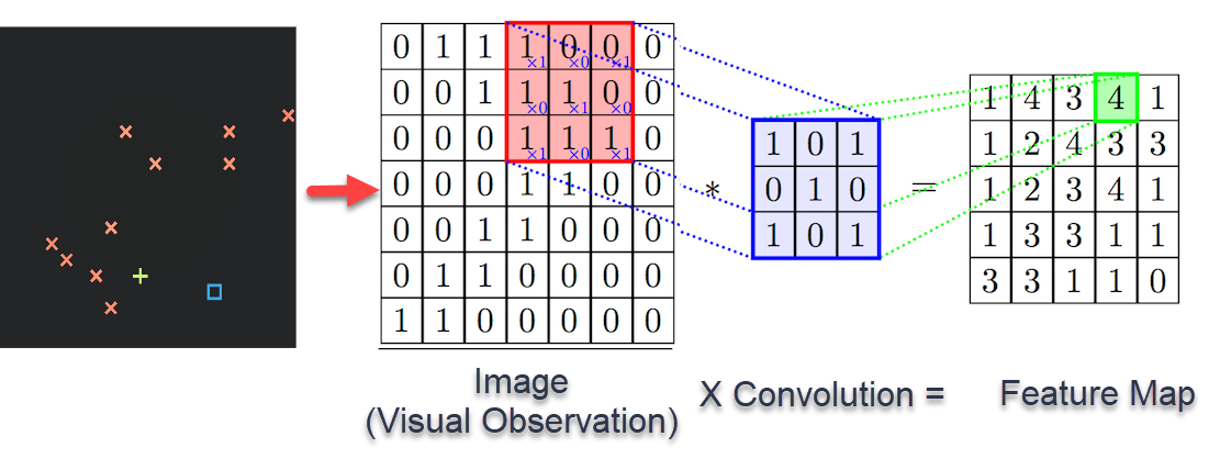
When processing visual data, it seems that to simply flatten the image and feed it as a vector is a bit disappointing. I mean, it works -- but remember what I said about the Bayesian prior? The network should a priori understand what the "inherent structure" of a data type is, so that it is more inclined towards more likely models.

The need for convolutional neural networks arises from this need to "bias" our network in favour of learning features that are more likely to be useful -- doing things that a Bayesian prior would do in lieu of actually having some Bayesian inference. More specifically, we want to represent the following prior knowledge about the features we want to learn:
  • "Features are based on local interactions" -- you are likely to be interested in linear combinations of neighbouring points. Further, there is a hierarchial nature to this, in that we are further interested in the interactions between nearby features, etc.
  • "Isotropy" -- the network shouldn't be overfitted for centered characters, etc. Even if it is, the bulk of the network should not be overfitted, i.e. relevant features should be identified throughout the image, and any overfitting that occurs in the last few layers can then be corrected through transfer learning (this is analogous to how humans learn, as well).
The second point corresponds to the idea of parameter-sharing ("basically all" points should undergo the same processing), and the first tells us that the exact kind of processing done should be based on local interactions, i.e. the precise notion of a convolution. Furthermore, the "hierarchial nature" of image processing leads to the notion of either pooling or stride, which brings distant features closer together. 

(Source: https://subscription.packtpub.com/book/game_development/9781789138139/4/ch04lvl1sec31/convolutional-neural-networks)

(Short project ideas: Check the claims above:
  • Garble/permute the rows and columns of the images and see how that affects the training accuracy with convolutional networks (make sure you apply the same permutation to all images!) 
  • Train a CNN on MNIST digits then do transfer learning on randomly off-centered digits with the convolutional layers fixed and check that you are able to get a similar accuracy to before. 
(Link to Colab Notebook where I perform these tests))

(Quick note: There are two forms of pooling, max-pooling, which tests for presence of a feature, and mean-pooling, which tests for sustained presence of a feature. Max pooling may be better if you don't have padding, otherwise it doesn't generally matter which form of pooling you use, as the convolution is capable of spreading a required feature to nearby pixels of a layer.)

In general, the notion that the fundamental operation of the neural network (affine transformations with vectors, convolutions with images) should depend on the "type" of the input data, is an important one. 

Once one understands that convolutions are the "fundamental way" of dealing with images, we should simply write convolutional neural networks in the abstract as any standard neural network, i.e. thinking of these "blocks of convolution kernels, plus bias kernels" as the appropriate generalization of "weights, plus biases".

Convolutional neural network: each block in the network is a vector of images, i.e. an image with channels.
A very important data "format" to care about is that of a data stream. This is something crucial to any AI that has a concept of time. All the data received by humans is in the form of a data stream, so it is easy to see that processing such data is important when attempting to replicate human tasks.

The natural structure on a data stream is given -- much like the natural structure on an image is given by notions of closeness -- by the flow of time. 

Note that simply intuiting the "structure" of the data type doesn't uniquely tell us what the network architecture should be. In fact, the cases of the convolutional and recurrent neural networks aren't even totally analogous -- recurrent neural networks are actually necessary for data streams, because of the input size not being fixed. Nonetheless, principles like parameter sharing are somewhat analogous in each context. 

Recurrent neural network architecture

The "parameter sharing" that goes on here is that the the parameters of each horizontal slice of the network are the same. Of course, here this parameter-sharing is required by the lack of fixed input size. It's also worth noting how this isn't analogous to convolutional networks, importantly: the information about nearby cells is fed into a layer by neurons in the same layer (as opposed to convolutions, which would have diagonal arrows). Nonetheless, the idea that our processing of a data stream is in some sense "consistent" or "uniform" over time somewhat motivates our understanding of this architecture.

Wrapped version of recursive neural network depiction. Input is a data stream.

(In this case, the unwrapped depiction is a better mental model when training the network, as the graph is acyclic, so you can apply backpropagation normally.)

"Bidirectional recurrent network", for updating your knwoledge/memory based on new information. This network has two "memory canals", carrying information forward as well as backward. The wrapping suppresses it in the depiction, but the second memory canal feeds into itself in the opposite direction as the data stream.


Data streams: Recurrent neural networks and Turing-completeness

One way to understand recurrent neural networks -- as we did above -- is as the natural algorithm for processing the specific data format called "data stream".

Of course, this isn't really "all there is", The precise structure of the recurrent neural network seems somewhat arbitrary, and it isn't truly completely determined by saying "it's the natural way to process data streams". Some genuinely new structure is seen here, and we should ask for a corresponding universal approximation theorem for recurrent networks.

The question to ask is: what exactly is the new structure seen in RNNs? How, precisely, is it different from standard feedforward networks?

A standard feed-forward network seeks to simulate functions, right? So the "universal approximation theorem" says that a neural network can approximate any function, up to something. So what does a recurrent neural network seek to simulate? What is a "function on a data stream"?

To answer this, we should talk about what exactly a function in the sense of computer science is. A function cannot really "take in a data stream" in computer science. A data stream that has not yet been fully fixed/captured is not a valid input variable, it's not a valid input data type.

What we're trying to simulate isn't really a function -- it's a program. A function is an example of a program, but a more general computer program can actually look at a data stream as it's running and continually update its output based on it. And the analog of universal approximation for programs is Turing-completeness, which RNNs do possess (as proven in [Siegelmann & Sontag, 1992]).

(A short project you can do to test the claim that RNNs indeed simulate programs: check that an RNN tested for a certain length of data input works reasonably well on inputs of different sizes. Can you do this with a CNN?)

You might get the sense that the RNN architecture we've discussed doesn't really feel the same as the way we process streams of data. It seems too generic, like there are more specific tasks we always do in our minds while processing some stream of audio or video. Like we need a better prior, to tell the network the exact nature of what it means to "mix" past and present features.

With the human mind, we have a very specific notion of memory -- specific actions to add and remove things from our memory. This construct is of importance, while watching a movie, holding a conversation, or reading a sentence. It's not just recalled memory, that is stored somewhere and accessed through searching for keywords in the mind, but actively held short-term memory that is particularly relevant in this context. During any of these activities, the human mind will never adopt any other "mixing" mechanism between knowledge from different points in time, that doesn't go through memory.

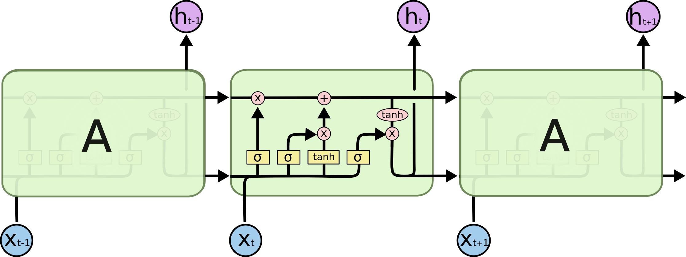
This is the idea behind Long Short Term Memory (LSTM) networks. Every recurrent "layer" of an LSTM network actually involves the following three computations:

  1. The forget filter -- based on current input, the network drops of some elements in the "memory channel" (called the cell state in LSTM)
  2. The remember filter -- the network adds some features of the current input to memory at varying intensities. 
  3. The output filter -- the network allows some of the current memory to pass to output.

I call these "filters" and use language like "dropping elements" and "some features", but it is to be noted that these are really about differences in intensity, and involve multiplying by the output of trainable sigmoid layers that decide how much of your memory/features you want to allow to pass through.

Source: Understanding LSTM networks by Christopher Olah

As an exercise, figure out which parts of the network correspond to which of the filters I've mentioned.

(Short project idea: I'm actually not completely sure if I understand whether the bottom channel is needed, i.e. whether its contents must be transfered to the next iteration in the sequence. Experiment with this alternative on standard applications of LSTM and compare the performance.)


Environment interaction: Reinforcement learning

With standard neural networks, feedback is specifically provided in the form of predetermined data and labels that the network is required to predict.

Reinforcement learning can be seen as a generalization of this, where the feedback isn't prepared by something complicated like a human, but instead is the result of dynamic interaction with an environment (or game). The environment typically follows some laws (i.e. the laws of physics, or the laws of a game -- for robotics and game bots respectively), and this automatically generates massive amounts of data, and computes an action's consequences, which act as a generalized notion of data "labels".

A problem is immediately clear with this method: how do you differentiate an environmental response against your network's parameters? This is not a minor technical problem -- differentiation fundamentally requires that you know what happens if you change your parameters a bit.

E.g. suppose you have a network that takes in the current state of a game and outputs a real number between 0 and 1, representing the probability that it tells the agent to "jump". Then you can differentiate each decision with respect to the parameters; however, you cannot differentiate the outcome (win/loss) with respect to the decisions.

The solution to this problem comes from recalling that we are trying to maximize an expected score, so we should be doing some sampling. More formally: we should play around with expectations.

Let $Y$ be the random variable representing the agent's decision (i.e. "jump" or "not") for some given input $x$, with probability function $P(Y|x, \theta)$ where $\theta$ is the network's trainable parameters. Then where $L(x, Y)$ is the environmental loss function, we are interested in minimizing $E(L)$.

\[\begin{align}
  {\nabla _\theta }E\left[ {L(Y)} \right] &= {\nabla _\theta }\sum\limits_Y^{} {P(Y)L(Y)}  \\
   &= \sum\limits_Y^{} {{\nabla _\theta }\left[ {P(Y)} \right]L(Y)}  \\
   &= \sum\limits_Y^{} {P(Y)\frac{{{\nabla _\theta }P(Y)}}{{P(Y)}}L(Y)}  \\
   &= \sum\limits_Y^{} {P(Y){\nabla _\theta }\left[ {\log P(Y)} \right]L(Y)}  \\
   &= {E_Y}\left[ {{\nabla _\theta }\left( {\log P(Y)} \right)L(Y)} \right] \\
\end{align} \]
So the solution is as follows: sample a large number of gameplays. Now pretend that each decision contributed directly to the victory and optimize them -- encourage all the moves in winning gameplays and all the moves in losing gameplays, i.e. update the parameters by the average value of $ {{\nabla _\theta }\left( {\log P(Y)} \right)L(Y)} $ across the sample.

So despite the bizarreness of pretending that every move in a winning play was correct and every move in a losing play was wrong, doing this for a large sample makes incorrect learned features cancel out -- a good move is expected to produce better results when all other moves are averaged out, and a bad move is expected to produce worse results when all other moves are averaged out.

This strategy is known as policy gradients, and is a general technique to deal with non-differentiable feedback.

Image source: Andrej Karpathy

(You may notice that this is incredibly inefficient. Indeed, this article only covers the most basic and superficial elements of cognition -- the human brain is capable of reasoning, and of producing a highly abstracted model of the game in its mind, and of transferring intuition from elsewhere onto the game.)


Generation: Generative (matching and adverserial) neural networks

Equipped with the ability to process data, the obvious next step is to get an AI to produce things -- to get an AI to be creative. To come up with art, compositions, original thoughts and ideas. We'll now describe the most elementary of such neural networks, which we will call Generative Neural Networks, while more complicated ideas would exploit some sort of transfer learning.

It's not at all absurd to expect it to be possible for a neural network to generate images of horses that don't look like any horse it's actually seen -- because humans can do that! If you imagine a horse, it's probably not a horse whose image you've seen before, but it nonetheless possesses the features you've identified as common between horses.

The idea behind a generative neural network can be motivated from the following two statistical notions:

  • The inverse transform method of generating random variables.

Content generated by a mind can be considered to be a random variable in some fancy space. E.g. if we want to get our neural network to produce (28, 28) digit characters, we're training it into a random variable on the space of (28, 28) images whose support is the images we identify as valid digit characters.

The way that computers typically sample random variables is through the "inverse transform method", which is to start with a uniform random sample and apply $F^{-1}$ to your sample where $F$ is the CDF of the random variable $X$ you want to sample. Your result will be a sample of $X$.

Quick explanation of inverse transform method: under the uniform distribution, the probability of getting a value under $u$ is $u$, which under the CDF of $X$ is the probability of getting a value under $F^{-1}(u)$. So you map $u\mapsto F^{-1}(u)$.
So we once again need a function approximator -- to approximate $F^{-1}$.

The inputs to the neural network are randomly generated, typically uniformly

  • A nonlinear generalization of principal component analysis

Think, e.g. of eigenfaces. If you've ever tried to use eigenfaces to generate realistic faces, you'll notice that your results are just terrible. Much of the information in faces is not so linear and nice -- there's no reason to expect it to be. Illumination and angle are pretty much the only properties that can be expected to vary linearly.

I.e. suppose you have some data that varies as follows:


Then a PCA might give you the pink line as your first principal component, but sampling from the pink line gives you a lot of unphysical outputs, those are the areas where your pink line doesn't intersect the data.

But using PCA to generate samples from a distribution can be understood as taking some random inputs, corresponding to the values of each principal component you want to use, and feeding them through a function, the principal component change-of-basis matrix. 

But more generally, replacing this function with something nonlinear allows us to deal with nonlinear models.

OK,so it's clear to us that we need a neural network -- a "generative neural network" -- to construct the inverse CDF. How would one train this network?

Given an initial random guess for the network parameters, what we have is some guessed distribution for "images of horses". And what we really want to do is perturb these parameters to match the distribution of our data.

Well, such an approach is certainly possible -- one could measure some notion of distance from our generated sample distribution and the real distribution and backpropagate this error with each iteration.

Note that we don't actually know the distribution of our data (the red one), so we can't really use something like "the probability of observing this sample given our distribution" as our loss function. Anyway, there are measures of the distance between two distributions that we could use for our error function, such as the maximum mean discrepancy approach, and methods involving moments.

(This approach, generally, is called a Generative Matching Network.)

But being arbitrary is generally disappointing in machine learning, and it's worth asking if there's a way to get the network to learn to discriminate between distributions.

Here's an idea: we could just subjectively tell that the outlier point did not belong to the distribution. We used our human brains. How about rather than defining a discrimination function, we trained a neural network to tell if a given data point could belong to a distribution? Then this neural network would train our generative neural network, and vice versa.

And this makes sense, right? When we learn to draw an object, we're also simultaneously learning to identify one.

And one could imagine showing off a generative network's results and having people guess if they're real or not (alongside actual real images of course) -- and based on whether they thought it was real, we could use it to train the network. These "people" are precisely what a discriminator network is.

In other words, we have two networks: the generator network, which generates random horse faces from random uniform variables, and the discriminator network, which takes the output of the generator network and some actual images, and figures out if the result is real or not.

If the classification is incorrect, the discriminator network is punished, while if it is correct, the generator network is punished.

This is known as a Generative Adverserial Network.

(add: GANN improvements [1], deepfakes, adverserial inputs)


Making connections: transfer learning

Something of crucial importance to human thought is the ability to make connections between ideas, transfering ideas and results from one area to another, either directly or by "abstracting out" the analogies.

There are many "levels" on which this occurs -- examples follow:
  • We don't need 60,000 instances to learn a script -- We can do with 1. It's shocking that we can learn distributional information from a single data point, and suggests that we already have an extraordinarily good prior. And we do -- our prior is continually updated from experience, of course, so this just means we're applying existing knowledge. We already know what features of the script are likely to be important and what can be safely discarded (hint: that accidental wiggle in the straight-ish line is probably noise) away. 
  • Prerequisites exist. So we depend on "applying" existing knowledge in some sense to learn new things. There's a reason why babies typically don't learn algebraic geometry. 
  • Making abstract connections between ideas -- Like recognizing that counting apples and counting sticks is the same task (and frivolous details about what an apple is or what a stick is can be lost for our purposes), recognizing that the algebra of kinematic quantities is the same to some extent as the algebra of quantum states (they both form vector spaces) (see Abstraction in mathematics, Abstraction in engineering), or recognizing the analogy between linear transformations of vector spaces and continuous functions of topological spaces (they're both categories).
There are probably multiple different algorithms in the brain that involve analogy and abstraction, and at least some of them (such as the first example above) have to do with learning.

This is the principle behind transfer learning, the idea that one may use the results of existing encoders for processing in other domains (and perhaps the precise encoder used may be fine-tuned for these other purposes). 

Examples of transfer learning architectures:


Progressive neural networks

This may be a bit of a disappointing solution to the question "How do brains think abstractly?" Our answer seems to depend on our active, hard-coded choice of what layers and encodings to preserve for our next task. Surely our brains do this somewhat "automatically" -- we don't actively tell our brain "Look, you've seen lines, remember? Well, there's lines here."

Well, maybe sometimes we do. It seems there may be some element of a conscious thought (whatever that means on an algorithmic level) in making analogies when it comes to complex intellectual tasks. But we certainly do not undergo any conscious thought when it comes to something like character recognition.

An architecture that may be analogous to our brain's cognition is that of a progressive neural network -- here, layers are algorithmically transferred from a previous task to another, with transferred parameters frozen. The picture below conveniently helps us make the analogy to "lateral thinking".

Source: arXiv:1606.04671

This architecture is capable of (and is about) choosing the sources of information that are most effective for the required task, but what suggests to me that this isn't what our brain does exactly is the parameter wastefulness and increasing level of model complexity (trainable parameters), which doesn't seem to be analogous with our method of learning, which seems to be more or less symmetric between learned ideas.

Multitask learning

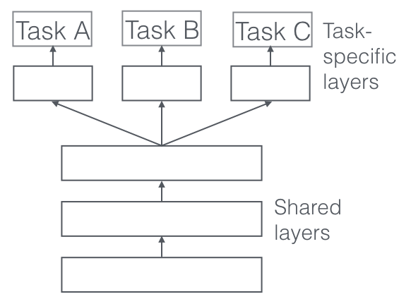
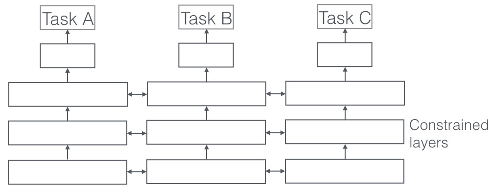
A far simpler transfer learning approach that addresses the above concern about symmetry is multi-task learning:
Hard parameter sharing. Source: Sebastian Ruder
Soft parameter sharing. Source: Sebastian Ruder

This does intuitively seem to be the brain's transfer learning algorithm -- even if one of the tasks has previously been trained, the brain seems to be able to retrain the network as needed. And I have often observed the benefits of learning two abstractly related areas of mathematics together, e.g. Hilbert spaces and quantum mechanics, linear algebra and special relativity, topology and probability theory.

Two ways to understand overfitting (and don't peek!)

Assorted comments on overfitting

The very first time I was introduced to the notion of overfitting -- by three diagrams of regression curves on scatter plots labelled as you may guess -- I became very uncomfortable. I was probably eleven years old, and did not understand Bayesian statistics, did not realize that seeing 51 heads out of a hundred didn't imply that the coin genuinely had a heads rate of 0.51.

Or rather: I didn't realize that I did realize that. If you had made me bet on the number of heads that would come up in the next hundred flips, I would not provide odds that would indicate an honest belief of seeing 51 heads.

(Because deep down, I had a non-uniform prior.)

And the same principle applies to drawing regression curves. You may insist that your curve with all its squiggles is "unbiased" or give any one of the terms (one for every squiggle) used to describe non-Bayesian estimators, but ultimately -- that's not the curve you'll bet on. You know it's just far more likely that those squiggles are the result of noise which will not be the same (or knowably correlated) in the next sample, than for them to actually be a determining feature.

Yes, maybe the 79th coin toss will always be a tail because of a tiny AI hidden in the coin that counts, or maybe it was the result of factors that affected the 79th coin toss that you just didn't measure. While your data should affect your beliefs, they shouldn't completely overrule your priors.

And that's the key idea behind overfitting (and really the Bayesian notion of probability in general) -- how will your model, based on your data, of perform if you exposed it to data it hasn't yet seen. Because using it on data it hasn't seen is the point of your model -- that is your purpose in building it.

So overfitting occurs when a model learns features specific to your particular data set that don't generalize well. There are two ways this can occur:

  • The training set is a biased sample: E.g. MNIST digits are all centered (but suppose you're testing on non-centered digits), or your medical database is all from a particular country. 
  • There is noise: I mean, of course there's noise -- it's a statistical problem. Even if the world were deterministic, you still don't have all the information in the world. And you should avoid your model using this noise to make predictions, since noise is, by definition, unpredictable.
The first is a more tractable problem -- it can often be solved by data augmentation (if you have a very good picture of exactly how the data set is biased) or transfer learning (if there's a good chance the model is picking up on important features so you can just train it on the ones it missed). It's important to develop interesting transfer learning algorithms to solve this anyway, as the way humans learn often involves biased samples (e.g. personal experience) and reasoning capacity to unbias their knowledge. 

(Not that humans do always do this -- people often do form beliefs based on mere personal experience, but humans are capable of reasoning more clearly.)

The second is a problem that requires algorithmic solutions that hint our neural network towards Bayesian solutions. Solutions like "well, parameters are just a priori unlikely to be very large, so let's penalize that" (Lasso/Ridge regression), or more complicated (to explain in a simple Bayesian way) regularization algorithms like cross-validation and early stopping.

Another unclassified comment on overfitting: it's very easy to mistakenly "peek" at the test data. Simply in the act of saying "hey, this model works well on the test data, let's choose it" you are already performing a simple algorithm that checks several models and chooses them based on their performance on the test data -- i.e. you are kinda training the model on the test data, even if it is not seen in your code, just in your choice of hyperparameters.

That's why developing some kind of "theory" of hyperparameter optimization and regularization techniques is of importance, so you actually have a theoretical justification for picking your models. 

(Of course, this is hard. We've always been picking models, haven't we? For example when we decide to model something as belonging to a particular family of distributions so we only have to optimize in a 1-dimensional parameter space instead of the literal theory-space. In a sense, machine learning is the way to avoid modeling, due to the universal approximation theorem -- and the hope is that we can eventually make the priors as human-like as possible, which is the eventual goal of hyperparameter optimization and regularization algorithms.) 

The Dirichlet (also Beta) distribution

Here's a category of distributions we may often want: a distribution on the simplex.

I.e. a multivariate distribution on $n$ nonnegative numbers that add up to 1. This is something that we can definitely see using as prior distributions on parameters that can be interpreted as "probabilities" of something. One can see that this is important for the Categorical and Multinomial distributions, for instance: and in the case of two numbers (i.e. a univariate distribution, since it's on a line segment), for the Bernoulli and Binomial distributions.

Here's one such distribution family that may come to your mind: for $x_i$ in the simplex $\sum_i x_i = 1$,

$$f(x_1,\dots x_n\mid\theta_1,\dots\theta_n)\propto \prod_{i}{x_i}^{\theta_i}$$
By adjusting the values of the $\alpha$s, one can get suitable priors that represent our beliefs correctly. This is known as the Dirichlet distribution, and its univariate case $f(x|\theta_1,\theta_2)\propto x^{\theta_1}(1-x)^{\theta_2}$ is known as the Beta distribution.

In fact the parameters of said distributions are usually provided a bit differently, with $\alpha-1=\theta$.

Exercise: Prove that:
  • The normalization constant is given by $\frac{\Gamma\left(\sum_i\alpha_i\right)}{\prod_i \Gamma(\alpha_i)}$
  • The mean is given by $E(X_i)=\frac{\alpha_i}{\sum_i\alpha_i}$
  • The Dirichlet distribution is the conjugate prior to the categorical/multinomial distribution. This is the key fact that makes the Beta/Dirichlet distribution important.

Poisson processes: from geometric to Gamma distributions

The notion of a Poisson process is rather beautiful, and connects a number of distributions together.

To start, consider a Bernoulli process: a discrete time series with each value IID Bernoulli. Then we can study some properties of this:
  • The waiting time for the 1st event is distributed geometrically. 
  • The waiting time for the nth event is distributed as the sum of geometric distributions, which is negative binomial.
  • The number of events in a given period of time is distributed binomially.
(You should be able to derive these distributions easily.)

(Note that this is not specific to a time series -- one has the same results for a spatial lattice or for some general abstract set of points.) 

How would one generalize this to continuous time? Well, with continuous time you really can't talk about the result for each point in time being "Bernoulli", or about them being IID. But let's do it anyway. Suppose an event has an $\mu\; dt$ chance of occurring in the timespan $dt$. Then the chance that the first event occurs at time $t$ is (by geometric distribution) ${(1 - \mu \;dt)^{t/dt}}\mu \;dt$, or: $\mu {e^{ - \mu t}}\; dt$, i.e. a probability density $\mu e^{-\mu t}$. This is called the exponential distribution.

The waiting time till the nth event is analogously just the sum of exponential random variables and its distribution can be computed through the standard MGF route. It is left as an exercise to the reader to show that the sum of exponential random variables with parameters $\mu_1,\dots\mu_\alpha$ is given by the Gamma distribution $\Gamma(\alpha,\sum\mu_i)$:

$$\Gamma(\alpha,\beta)\sim \frac{1}{(\alpha - 1)!}\beta^\alpha t^{\alpha-1}e^{-\beta t}$$
What does our notion of independence translate to? The idea that there being an event at some time should not depend on whether there was at any other time. Well, the natural way to write independence in a way that makes sense for continuous distributions is to consider the waiting time for the first event

\[P(T>t+s|T>t) = P(T>s)\]
This is known as memorylessness. Indeed, one can check that the only memoryless discrete distribution is geometric, and the only memoryless continuous distribution is exponential.

OK -- what about the number of events in the continuous case? Well, in some interval of size $T$, the probability of the number of events equaling some $n$ is (by binomial):

\[\left( {\begin{array}{*{20}{c}}
  {T/dt} \\
  n
\end{array}} \right){(\mu \,dt)^n}{(1 - \mu \,dt)^{T/dt}}\]
Which it is easy to see that equals:

\[\frac{{{{(\mu T)}^n}{e^{ - \mu T}}}}{{n!}}\]
Which is the Poisson distribution with rate parameter $\mu T$.

Here's a table of analogies between memoryless discrete and continuous processes:

Discrete time Continuous time
Overall phenomenon Bernoulli process Poisson process
Single-event Bernoulli distribution -
Waiting time (1st event) Geometric distribution Exponential distribution
Waiting time (nth event) Negative Binomial distribution Gamma distribution
Number of events Binomial distribution Poisson distribution

But isn't the continuous analog of the binomial distribution (and many other distributions) the normal distribution? Do not conflate discrete time with discrete number. Both the binomial and Poisson distributions above are discrete distributions: the Poisson is just the relevant one for the continuous-time process. These are completely unrelated notions.

Probabilistic inequalities

Consider a random variable with mean 0 and variance 1 (this is like the "natural units" of second-moment probability). Now this variance puts a value on how dispersed the PDF of the random variable can be: one couldn't, for example, have two Dirac-delta poles really far from the origin, because you can calculate the variance of that, and it's too high.

Which raises the question: for some $k$, what's the maximum fraction of the distribution that can be outside $(-k,k)$?

Ok, one thing is clear: at this maximum, there should be nothing outside $[-k,k]$, because then you could bring inwards without changing the fraction but reducing the variance.

Also, for any value in $(-k,k)$, if you moved it over to the mean (0), the variance would go down. So the distribution must be comprised of just three poles at 0, $-k$ and $+k$, and is necessarily symmetric so that the mean is at 0. Letting $p/2$ be the height of each pole at $k$, the variance in terms of $p$ is $pk^2$. So $pk^2=1$, and $p=1/k^2$. I.e.

$$P\left(\left|X\right|>k\right) \le 1/k^2$$
Or for general mean and variance:

$$P\left(\left|\frac{X-\mu}{\sigma}\right|>k\right) \le 1/k^2$$
This is Chebyshev's inequality, and gives you a limit on how much of the distribution can be some given distance $k$ from the mean. Note how it only becomes interesting for large $k$ ($k>1$).

Well, clearly this approach seems to open up a whole world of similar inequalities. Another is the Markov inequality, which states that (for a nonnegative random variable) no more than $1/k$ of a population can have value more than $k$ times the mean, i.e.

$$P\left(X\ge k\right)\le\frac{\mu}{k}$$
(Justify this with similar reasoning as Chebyshev's.)

In fact, Chebyshev's inequality can be derived as a special case of Markov's (do it).

The point of these inequalities is that means and variances are generally easy to track, even when probability distributions are unknown. Providing bounds on probability fractions based on these is very useful for proving convergence in probability -- for example, the weak law of large numbers becomes elementary with Chebyshev's inequality.

Probabilistic convergence

The law of large numbers is something that we know, that in our heads is almost the definition of probability (it's not): "as sampling increases, the average of a variable approaches its expected value". I.e. for $X_i$ IID:

$$\lim_{n\to\infty}\frac1n \sum{X_i}=\mu$$
Let's think about what this statement really says: when you take more and more readings of $X$, the average will go closer and closer to $\mu$. But the values of these readings are inherently probabilistic: this is not an actual sequence of real numbers you can take the limit of. Rather, you are talking saying that of all the possible realizations (which are real number sequences), almost all of them (probabilistically) converge to the thing. I.e.

$$\mathrm{Pr}\left[\lim_{n\to\infty}X_n=X\right]=1$$
This is known as almost sure convergence.

In general, the thing on the right could've been a random variable, rather than a real number. And here's where some probability theory (read the article) comes in, because the random variables $X_n$ and $X$ need to be defined on the same sample space for this to make sense (i.e. it's not just about the distribution).

But with this, the definition as above still works: as an example, consider the sample space $[0,1]$ and consider a sequence of random variables $X_n$ that is respectively 1 on some corresponding sequence of sub-intervals approaching $[0,1/2]$. Then this approaches the random variable that is 1 on $[0,1/2]$ almost surely.

And yes, this is entirely due to the correlations between these things.

In any case, almost sure convergence isn't really the best way to express random variables converging to each other, as you can see. E.g. the central limit theorem -- like $\frac{1}{\sqrt{n}}\sum\frac{X_n-\mu}{\sigma}\sim N(0,1)$, cannot be phrased in terms of almost sure convergence, because $N(0,1)$ is a distribution, not a random variable.

Indeed, you may have figured that the problem of a random sequence converging to a random variable is somewhat similar to the notion of "functions converging to a function" -- indeed, one may think of the distributions of the random variables in the sequence and discuss their convergence. I.e.

$$F_n(x)\to F(x)$$
This is called convergence in distribution.

While convergence in distribution does not imply almost sure convergence in general as we've seen, we would expect that it does imply it in the case where the limiting random variable is constant (because then issue of correlations disappears).

But you may realize that this is not really so: a sequence may look increasingly like something without actually limiting to it. For example, think about a sequence like 1, 1, 0, 1, 0, 0, 0, 0, 1, 0, 0, 0, 0, 0, 0, 0, 0, 0, 0, 0, 0, 0, 0, 0, 0, 1... with an infinite number of 1s, but decreasing in frequency. This doesn't limit to zero. If this were a deterministic sequence, this would never be expected to limit to 0 as the positions of the 1s would be hardcoded into the generation of the sequence. However, the sequence can also be realized as a realization of a sequence of random variables $X_n$ that have probability $1/n$ of being 1. Then the $X_n$ converge in distribution to 0, but their realizations almost never (thus in particular don't almost surely) converge to 0.

So it seems that asking for realizations to almost surely converge to the right thing is a bit too strong for a lot of purposes. A weaker notion of convergence than almost sure convergence can be constructed by considering probabilities of each $X_n$ separately rather than as a sequence: $X_n$ converges to $X$ if each $X_n$ is in the limit almost surely arbitrarily close to $X$. Or more precisely:

$$\lim_{n\to\infty}\mathrm{Pr}\left(\left|X_n-X\right|<\varepsilon\right)=1$$
This is known as convergence in probability. Indeed:
  1. Almost sure convergence implies convergence in probability (obviously).
  2. Convergence in probability implies convergence in distribution (because they are both topological notions of convergence and the map from a random variable to its distribution is continuous).
  3. When the limit random variable is constant, convergence in distribution implies convergence in probability.
In fact, the law of large numbers that we stated above (in terms of almost-sure convergence) is the strong law of large numbers, while the weak law of large numbers only states convergence in probability.


Exercise:

Prove Slutsky's lemma: given $X_n, Y_n$ converge to $X,y$ in probability and $y$ is a constant random variable:

  1. $X_n+Y_n$ converges to $X+y$ in probability.
  2. $X_nY_n$ converges to $Xy$ in probability.
  3. $X_n/Y_n$ converges to $X/y$ in probability.
Why is it necessary that $y$ be a constant?

I don't believe p-hacking is a problem.

Or more precisely: I don't believe p-hacking is a fundamental mathematical or statistical issue, but rather an issue with the methods adopted by experimental researchers.

If you haven't heard of p-hacking, it's as follows: suppose you want to find predictors for cancer. You test 100 possible predictors each at p-value 5%. Now although the chance of a false positive on any given test is 5%, you're expected to get 5 false positives in the test. So you can "always" find a (fake) predictor for cancer just by surveying enough things.

Another way of putting it: even if your factors don't actually predict cancer, the probability distribution for the observed correlation for any one factor may look something like this.

So when you test for these factors, when the correlations you observe actually sample the above curve, you're faced with a question: do you believe the points that lie in the shaded region (beyond your significance level) actually reject the null hypothesis?

On one hand: they lie beyond your significance level. Individually, you need to reject those null hypotheses.

On the other hand, one can also think of a "mega-" null hypothesis as implying the above curve: since your points sample the curve, you need to accept the null hypothesis.


I believe the answer is to reject those null hypotheses, i.e. to not make any "corrections" for having tested multiple parameters.

Here are some explanations:
  • An individual researcher "p-hacking" is fundamentally/mathematically no different from a large number of researchers investigating of various different parameters. Surely it makes no sense to argue that all positive results in the literature should be ignored, or that they should be evaluated at much stronger significance levels. 
  • When you investigate a large number of parameters, the probability of a true positive is also higher (in a Bayesian sense). If your positives are more likely to be false than true when you're testing a hundred parameters, they were more likely to be false than true when testing one parameter too. Of course, you are much more likely to have false positives when testing more parameters, but that doesn't increase the chance that any given deduction is false, because there are more true positives, too. 
  • Or in other words, the "mega-null hypothesis" probably isn't true. If the $\theta$ parameters are independent, then you'll probably have a large number of false null hypotheses. The "mega-null hypothesis" argument actually seems to assume zero probability of a true positive. 
  • Equivalently: just apply Bayes's theorem/the fact that probability is commutative. (equivalent to the first point)
Also note how the Bonferroni correction has nothing to do with p-hacking: it applies to looking at probabilities/confidence levels of several hypotheses being true, not about one.


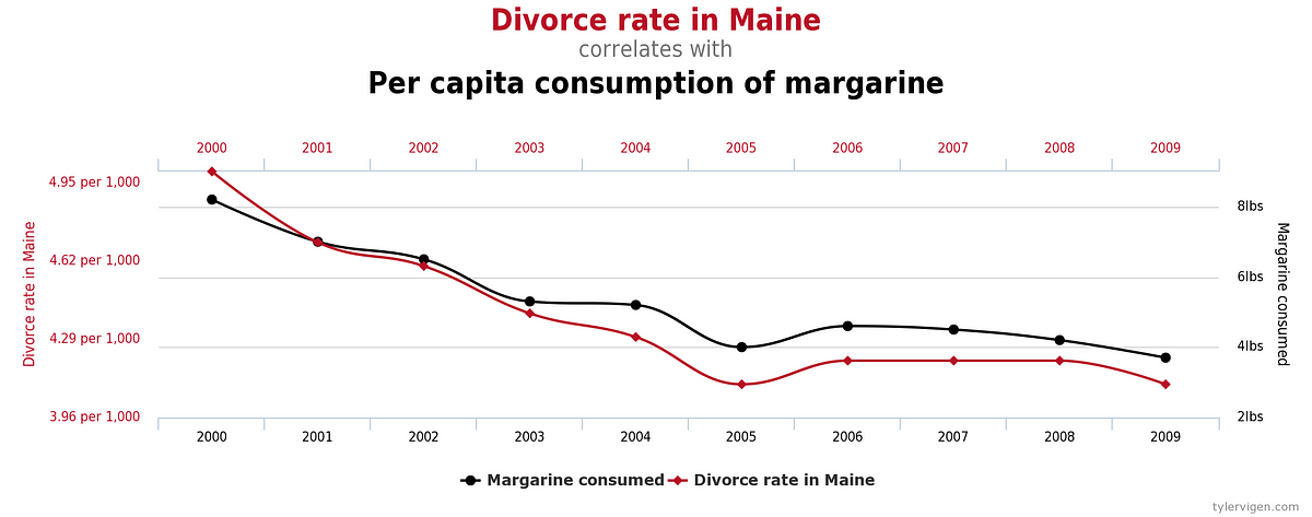
So, then, why do the consequences of p-hacking all seem to bizarre? Stuff like this:


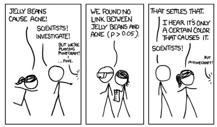
Or this:

Full comic for context: xkcd 882
Surely we don't actually believe that margarine causes divorces in Maine, or that only green jelly beans cause acne?

And no, we don't.

Why not?

Because there is no a priori reason to suspect that margarine causes divorces in Maine. Because a priori, we know that it's highly likely that whether green jelly beans cause acne is correlated with whether all the other color of jelly beans cause acne (because it's very unlikely that colour itself causes acne). These correlations should be embedded in our prior.

But these aren't fundamental issues with the nature of statistics. These are issues with how frequentist researchers may often decide which hypotheses to test. One should have some theoretical justification to formulate a hypothesis: that's how you know the prior probability is significant. Unless you have a good theoretical model for why a certain correlation/etc. should hold, the hypothesis should not be tested.

This problem is particularly prevalent in the social sciences, where a "general mathematical theory" of social science does not exist. Even in economics, you often end up with pseudo-science like this: Want to expand the economy? Tax the rich! (this particular study was terrible on several levels: (1) the conflation of correlation and causation -- this is always a problem when you have temporal trends, because time is a hidden parameter; that's why you should do cross-sectional studies (2) the correlation was statistically insignificant by any standard (3) there was no theoretical justification for why progressive taxation would expand the economy, leading to the problems discussed in this post.)

This point is essentially the point made by several papers (links: [1][2]) discussing "multiple comparisons in a Bayesian setting" -- it is what is meant by claims like "the multiple comparisons problem disappears when you use a hierarchial Bayesian model with correlations between your parameters".

Classical Statistics, Confidence Regions and Hypothesis tests

The basic general idea behind a confidence region is this: Given that the true value of some parameter is $\theta$ we may have some mechanism to sample "random regions" $R$ for $\theta$ such that 95% of these random regions contain $\theta$.

The first obvious issue is that this mechanism should not depend on $\theta$, as it is not known to us. We want a general experimental mechanism that for any $\theta$, produces random regions of the same confidence level ("95%").

In some basic cases, this is easy: for example, suppose we have some $X\sim N(\mu, 1)$. Then for any $\theta$, 95% of intervals generated as $X\pm 1.96$ contain $\mu$.

The key hint that you may find in the example above is that $\mu$ is a location parameter for $X$, i.e. the probability of $X\mid\mu$ is a function of just $X-\mu$, i.e. the distribution of $X-\mu$ itself does not depend on $\mu$, and is just $N(0,1)$. $X-\mu$ is what we call a pivotal quantity here.

In general, a pivotal quantity is a function of some data and the true value of the parameter itself $k(X,\theta)$ such that its distribution is completely specified. Then a confidence region for $k$ can hopefully be transformed back into a confidence region for $\theta$ at the same confidence level.


OK, next question: what is the implied prior of confidence region calculations? I.e. under what prior can the confidence level be interpreted as the probability that the true value of the parameter is contained in the confidence region?

(For a general prior, such a region that gives you some probability of containing the true value of the parameter is called a credible region.)

Well, what exactly is the confidence level? It's the probability that a randomly generated random region contains the true parameter value -- i.e. before you actually know what the random region is. Once you get the generated random region, this probability may change depend on the prior probability of the true parameter value being in this concrete region.

In other words, the implied prior is one such that $\theta$ has an equal prior probability of being in any possible confidence region. This is easy to calculate in some specific examples:
  • If $\theta$ is a location parameter for $X$, the implied prior on $\theta$ is uniform, $\propto 1$.
  • If $\theta$ is a scale parameter for $X$, the implied prior on $\theta$ is logarithmic, $\propto 1/\theta$.  


The way that hypothesis testing is first introduced, one talks of things like "the probability of finding a value of $x$ at least as extreme as you did". And one sometimes chooses a "one-sided" hypothesis test and other times a "two-sided" hypothesis test. It should be clear that this isn't too fundamental a concept to be interested in.

Rather, one sensible, more generally appropriate way of thinking of hypothesis tests is in terms of confidence regions. Specifically: testing a null hypothesis is equivalent to asking if it is contained within the confidence region of our data.

Obviously, this depends entirely on the shape we choose of our confidence region. We can always just choose a confidence region that includes or excludes our null hypothesis and maintain the same confidence level.

While it may be disappointing that there is no one way to construct a confidence region, this makes a great deal of sense. For example, consider the following multimodal distribution:


The sensible confidence region to construct would then be one that contains the bulk of both peaks. "Sensibility" in this sense is getting the confidence region of the least length (you may observe that this is not reparameterization-invariant).

Various different constructions of confidence regions is what gives you things like two-tailed and one-tailed tests.

Also read: Choosing the more likely hypothesis by Richard Startz

Matrix decompositions

Some decompositions

The algorithms for the QR and LU decompositions are fairly self-explanatory from their definition.

The Cholesky decomposition can be computed for a nonnegative-definite matrix through a simultaneous LU decomposition from both sides. Starting with a matrix in the block form:

\[A = \left[ {\begin{array}{*{20}{c}}
  {{a_1}}&{{v^T}} \\
  v&{{A_2}}
\end{array}} \right]\]
We perform an LU decomposition first on the columns, from the left, then on the rows, from the right:

\[\begin{gathered}
  \left[ {\begin{array}{*{20}{c}}
  {{a_1}}&{{v^T}} \\
  v&{{A_2}}
\end{array}} \right] = \left[ {\begin{array}{*{20}{c}}
  {\sqrt {{a_1}} }&0 \\
  {v/\sqrt {{a_1}} }&1
\end{array}} \right]\left[ {\begin{array}{*{20}{c}}
  {\sqrt {{a_1}} }&{{v^T}/\sqrt {{a_1}} } \\
  0&{{A_2} - v{v^T}/{a_1}}
\end{array}} \right] \\
   = \left[ {\begin{array}{*{20}{c}}
  {\sqrt {{a_1}} }&0 \\
  {v/\sqrt {{a_1}} }&1
\end{array}} \right]\left[ {\begin{array}{*{20}{c}}
  1&0 \\
  0&{{A_2} - v{v^T}/{a_1}}
\end{array}} \right]\left[ {\begin{array}{*{20}{c}}
  {\sqrt {{a_1}} }&{{v^T}/\sqrt a } \\
  0&1
\end{array}} \right] \\
\end{gathered} \]
The process can then be continued to give an LU decomposition where the $L$ and $U$ are transpose, thus the Cholesky decomposition.

(Why does the matrix have to be nonnegative-definite?)

Eigenvalue algorithm

A lot of factorisations are fundamentally related to the "eigen"-stuff: this includes the change-of-basis factorizations: diagonalization, SVD, Schur -- and also the polar decomposition. Eigenstuff is fundamentally analytic (whatever that means), so terminating algorithms won't work, we need an asymptotic algorithm.

A simple such algorithm to calculate the eigenvectors and eigenvalues is power iteration. It is related to the flows of systems of linear differential equations, in which the eigenspace with the largest eigenvalue provides the only stable equilibrium of the system. Unless you choose an initial vector $v$ that happens to itself be an eigenvector, $A^nv$ will approach the projection of $v$ onto the principal eigenspace of $A$.

So that gives you the largest eigenvalue. There are many ways to get the remaining eigenvalues -- one inefficient way I thought of was to subtract off the part corresponding to the stretching of the primary eigenvector, but this is incredibly inefficient and numerically unstable.

An actually sensible approach is as follows: consider the matrix $(A-\mu I)^{-1}$, which has the same eigenspaces as $A$. The largest eigenvalue of this is the eigenvalue of $A$ closest to $\mu$. By varying $\mu$ across the real line, one can discover all the eigenvalues of $A$.

Schur algorithm

You can use the eigenvalue algorithm to calculate the Schur decomposition directly via its definition -- however, there is a more efficient method.

A triangular matrix is invariant under conjugation by the $Q$ in its own $QR$ decomposition (because the $Q$ is the identity matrix). So similar to power iteration, one may iteratively QR-factorize $A$ and replace it with $RQ$. This is called the QR algorithm.

Apparently this is expensive in its crude form, so you instead bring into a form called "upper Hessenberg form" (upper-triangular but with a subdiagonal) and that apparently makes the computations less expensive. The mechanism to bring a matrix into upper Hessenberg form is based on householder reflections, and involves doing householder reflections on the parts of the columns below the subdiagonal, so the corresponding householder reflections on the rows (since the Schur is a change-of-basis transformation) do not interfere with the column of interest and screw up all your zeroes. It's not very interesting.

Least-squares

Suppose you wanted to solve $Ax\approx b$, i.e. find the $x$ that minimizes $\|Ax-b\|$. This is relevant when $A$ is not surjective.

The idea is that $\|Ax-b\|$ is minimised when $Ax$ is the projection $b_A$ of $b$ onto the image of $A$. One can equivalently write $A^{T}(Ax-b)=0$, as $Ax-b$ is perpendicular to the column space of $A$. Thus it suffices to solve $A^TAx=A^Tb$.

If $A$ is full-rank (this does not mean surjective), we can actually have a unique $x$, given by $x=(A^TA)^{-1}A^Tb$, and $A^+=(A^TA)^{-1}A^T$ is called the "Moore-Penrose pseudoinverse" of $A$.

An alternative, more efficient algorithm is to use the QR factorization (the one with the non-square $Q$) to construct the projector as $QQ^T$ (which works, as $Q$ definitionally provides a basis for the image, and $QQ^T$ satisfies the defining property of a Hermitian projector). Then one can solve $QRx=QQ^Tb$, or equivalently $Rx=Q^Tb$. In the full-rank case, $R^{-1}Q^T$ is the Moore-Penrose pseudoinverse.

To add:
  • SVD algorithm
  • Algorithm complexity for each thing