Information and bits

When we deal with questions of statistical inference, we often talk in terms of information -- we say that an observation provides information, that interferes through the Bayes mechanism with our prior distribution to form the posterior.

But what exactly does "information" mean? Surely there must be a way to quantify it, to be able to compare two sources of information based on the "amount" of information they provide.

Well, consider our sample space, say for an experiment that involved tossing three coins:

$$\{HHH, HHT, HTH, HTT, THH, THT, TTH, TTT\}$$
"Information" would be something like the statement "the first toss was a heads", or "the first two tosses yielded different results", or "the tosses were not all heads". This is information, because this narrows down our sample space. So we can think of information as being quantified by the fraction of hypotheses eliminated, or more precisely: the fraction of probability mass eliminated.

"But statistical inference isn't just about eliminating hypotheses!" It kind of is, actually. Observations are about restricting your sample space, i.e. completely eliminating specific possible observations. I.e. even when applying Bayes's theorem $P(Y|X=x)=P(X=x|Y)P(Y)/P(X=x)$, the statement $X=x$ is a certain fact, and all inferences made through Bayes's theorem are a recalculation of probabilities on this restricted sample space.

It's generally common (for reasons that will become obvious later in the article on data compression) to represent the amount of information in terms of bits.

Each bit of information eliminates half the probability mass upon being found to be true. 

Intuitively, one may imagine that we're attempting to identify some data in the form of a binary sequence 11001????????... where each sequence has an equal probability. Discovering one new bit halves the space of possible sequences. Of course, our data may not be in this form, something we will get to in the data compression article.

Or in general, the quantity of information carried by an observation $X=x$ is defined as:

$$I(X=x)=\log_{1/2}(P(X=x))$$
So this notion of information captures our intuitive idea that "the unlikelier a fact seems, the more information it will provide us if it turns out to be true/the more it will change our beliefs".

I don't believe p-hacking is a problem.

Or more precisely: I don't believe p-hacking is a fundamental mathematical or statistical issue, but rather an issue with the methods adopted by experimental researchers.

If you haven't heard of p-hacking, it's as follows: suppose you want to find predictors for cancer. You test 100 possible predictors each at p-value 5%. Now although the chance of a false positive on any given test is 5%, you're expected to get 5 false positives in the test. So you can "always" find a (fake) predictor for cancer just by surveying enough things.

Another way of putting it: even if your factors don't actually predict cancer, the probability distribution for the observed correlation for any one factor may look something like this.

So when you test for these factors, when the correlations you observe actually sample the above curve, you're faced with a question: do you believe the points that lie in the shaded region (beyond your significance level) actually reject the null hypothesis?

On one hand: they lie beyond your significance level. Individually, you need to reject those null hypotheses.

On the other hand, one can also think of a "mega-" null hypothesis as implying the above curve: since your points sample the curve, you need to accept the null hypothesis.

---

I believe the answer is to reject those null hypotheses, i.e. to not make any "corrections" for having tested multiple parameters.

Here are some explanations:

• An individual researcher "p-hacking" is fundamentally/mathematically no different from a large number of researchers investigating of various different parameters. Surely it makes no sense to argue that all positive results in the literature should be ignored, or that they should be evaluated at much stronger significance levels. 
• When you investigate a large number of parameters, the probability of a true positive is also higher (in a Bayesian sense). If your positives are more likely to be false than true when you're testing a hundred parameters, they were more likely to be false than true when testing one parameter too. Of course, you are much more likely to have false positives when testing more parameters, but that doesn't increase the chance that any given deduction is false, because there are more true positives, too. 
• Or in other words, the "mega-null hypothesis" probably isn't true. If the $\theta$ parameters are independent, then you'll probably have a large number of false null hypotheses. The "mega-null hypothesis" argument actually seems to assume zero probability of a true positive. 
• Equivalently: just apply Bayes's theorem/the fact that probability is commutative. (equivalent to the first point)

Also note how the Bonferroni correction has nothing to do with p-hacking: it applies to looking at probabilities/confidence levels of several hypotheses being true, not about one.

---

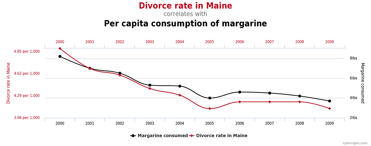
So, then, why do the consequences of p-hacking all seem to bizarre? Stuff like this:


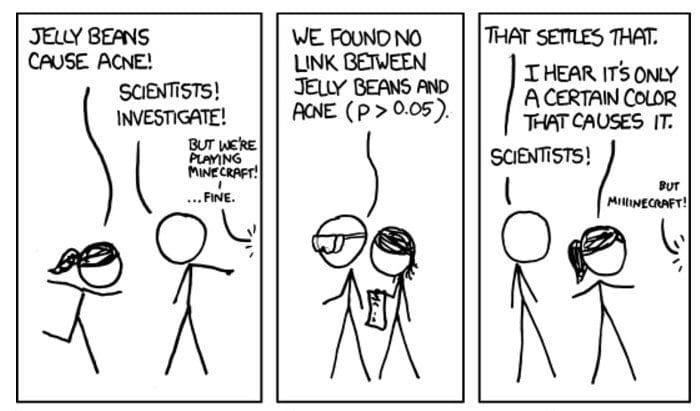
Or this:

Full comic for context: xkcd 882

Surely we don't actually believe that margarine causes divorces in Maine, or that only green jelly beans cause acne?

And no, we don't.

Why not?

Because there is no a priori reason to suspect that margarine causes divorces in Maine. Because a priori, we know that it's highly likely that whether green jelly beans cause acne is correlated with whether all the other color of jelly beans cause acne (because it's very unlikely that colour itself causes acne). These correlations should be embedded in our prior.

But these aren't fundamental issues with the nature of statistics. These are issues with how frequentist researchers may often decide which hypotheses to test. One should have some theoretical justification to formulate a hypothesis: that's how you know the prior probability is significant. Unless you have a good theoretical model for why a certain correlation/etc. should hold, the hypothesis should not be tested.

This problem is particularly prevalent in the social sciences, where a "general mathematical theory" of social science does not exist. Even in economics, you often end up with pseudo-science like this: Want to expand the economy? Tax the rich! (this particular study was terrible on several levels: (1) the conflation of correlation and causation -- this is always a problem when you have temporal trends, because time is a hidden parameter; that's why you should do cross-sectional studies (2) the correlation was statistically insignificant by any standard (3) there was no theoretical justification for why progressive taxation would expand the economy, leading to the problems discussed in this post.)

This point is essentially the point made by several papers (links: [1][2]) discussing "multiple comparisons in a Bayesian setting" -- it is what is meant by claims like "the multiple comparisons problem disappears when you use a hierarchial Bayesian model with correlations between your parameters".

Uniform priors and Maximum Likelihood Estimation

In the last article, we saw that Bayes's theorem allows us to infer theories from data -- or rather infer from data a distribution on the theory-space. This is the general way to make inferences and use these inferences to make predictions. We don't really need to bother about questions of whether we should choose the mean or median or mode as the theory we "choose", because we don't have to choose -- we make predictions with the entire distribution.

For example in the most general setting, we're trying to calculate our optimal action out of a set of choices based on a certain unknown utility function that depends on the right theory of physics (to calculate the consequences of the action). We don't need to "choose" the right theory of physics from the probability distribution we have on it -- we just make predictions for each possible theory in the support and integrate over the distribution to calculate the distribution on possible consequences. It's only at this point where we need to care about whether we want the action with the maximum mean, median, mode or whatever of the utility function.

Can you show that Bayesian inference can always converge? I.e. that there is always some data collection mechanism that allows your distribution to converge to a Dirac delta at some point? Well, there is, and it's called "sampling". What if we can't sample directly but collect some other indirect data? Comment on the philosophical implications of such a theory-space (hint: think about a probabilistic generalisation of falsifiability (a criterion for a theory to be scientific)).

But some special cases of Bayesian inference -- with special choices of prior -- exist and are often discussed/used in the literature for various reasons, and in fact, they often come with mechanisms to choose specific estimates based on the posterior distribution, as well as specific projections of our data to use. We will discuss some of these examples below.

---

Perhaps the most straightforward example is maximum likelihood estimation. Here, the prior distribution is the uniform distribution, i.e.

$$\mathrm{Pr}(\theta\mid x)=\frac{\mathrm{Pr}( x\mid\theta)}{\mathrm{Pr}(x)}$$
And we always take the mode of this (the value of theta that maximises $\mathrm{Pr}(\theta\mid x)$) to be the estimate of the parameter. This is just the value of theta that maximises $\mathrm{Pr}( x\mid\theta)$ (for observed data values $x$), which is called the likelihood function.

I.e. we're saying we have no preconceptions about the theory, and the right theory is just the one that gives the observed data the highest probability (or probability density).

Note that even in maximum likelihood estimation, you kinda do have non-uniform prior, in the sense that the prior is only uniform on its support, and you give zero values to things outside the domain of the parameter, or to theories other than the family being tested, etc. So if you were just taught maximum likelihood estimation, it would be easy for you to come up with the idea of Bayesian inference.

---

Suppose you have a prior distribution given by $\rho(\theta)$ and some specific value of $\theta_0$, which, regardless of the actual value of the prior distribution, you are "decisively" biased towards for some reason (e.g. you're looking at a suspect's guilt and you'll act on the assumption of innocence as long as the probability of his innocence is at least 1%). You may also be happy to consider a small neighbourhood around $\theta_0$ as "effectively" the same as $\theta_0$ for any practical purposes you may have (e.g. no coin is perfectly fair, but most coins are pretty fair).

Two-envelopes problem: beyond the Bayes explanation

The two-envelopes problem is phrased as follows:

There are two envelopes, one with twice the amount of money as the latter -- you pick one of them at random and open it to find $x$ dollars. You don't know if this was the larger or smaller sum.

Should you switch?

Though symmetry would tell you that it doesn't matter, it seems that by switching you get $x$ if the other envelope is bigger, but only lose $x/2$ if the other envelope is smaller. So you should switch. Right?

The standard explanation to this problem is that we need to pick a prior to make any actual inference, and the probability of the other envelope being bigger is usually less than the probability of it being smaller, in the sense that probability distributions approach zero towards infinity.

But this explanation doesn't really make the problem go away. Consider this prior:

$$
f(x) = \left\{ {\begin{array}{*{20}{c}}{\frac{1}{4}{{(3/4)}^n}}&{{\rm{if }}\ x = {2^n},\,\,n \in {\mathbb{Z}_{ \ge 0}}}\\0&{{\rm{else}}}\end{array}} \right.
$$
This is a perfectly valid prior distribution (the improper prior assumed in the original "paradox" would have worked as well, but I don't want to distract you with questions about distribution propriety) for which exactly the same paradox applies -- one may show (and I encourage you to work this out) that whatever value $x$ I find in the envelope, the expected value of the other envelope is $8/7\ x$.

Let's try to remember why this is weird -- what exactly is so paradoxical about it?

What's weird is that before opening your envelope, the situation is completely symmetrical. Yet you know that when whatever happens once you open the envelope, you'll want to switch.

Well, that's weird, but the reason it's paradoxical is this: since each expectation $E(X_2\mid X_1=x_1)$ (for varying possible $x_1$) is greater than $x_1$, the expectation of $X_2$ should itself be greater than the expectation of $X_1$, right? It's a tree diagram, you're just summing over each possible value of $X_1$.

How can $E(X_2)=8/7\cdot E(X_1)$ but at the same time $X_1$ and $X_2$ are completely symmetric?

Hopefully some light bulbs are turning on in your head -- indeed:

$$E(X_1)=\sum_{n\in\mathbb{Z}_{\ge0}}\frac14\left(\frac34\right)^n2^n=\infty$$
Yep. That's why the situation is symmetric. Because eight sevenths of an infinity is still an infinity.

Introduction to Bayesian inference

When the Higgs boson was discovered by the LHC, you heard comments e.g. here that "there is no way to definitively talk about the probability of the existence of a Higgs boson" -- more specifically, the quoted physicist in the linked article claimed "there is no way eliminate the conditional".

This is just wrong. There is a way to eliminate the conditional -- it's just Bayes's theorem!

Imagine setting up a tree diagram for this experiment. (The LHC made a certain observation which is highly correlated with the existence of the Higgs boson, which is what we're expressing below.)

As a graphical interpretation of Bayes's theorem:

$$\mathrm{Pr}(\mathrm{Theory}\mid\mathrm{Data})=\frac{\mathrm{Pr}(\mathrm{Data}\mid\mathrm{Theory})}{\mathrm{Pr}(\mathrm{Data})}\mathrm{Pr}(\mathrm{Theory})$$

What this needs, however, is a prior distribution $\mathrm{Pr}(\mathrm{Theory})$ on the probability of the Higgs boson existing -- before any data is supplied.

And this distribution obviously exists. If you've ever heard a physicist say "we were already pretty sure it existed, this experiment just increased our confidence in it", then you know what I'm talking about. This "pretty sure"-ness in its existence is a prior distribution.

OK -- but how does this prior distribution exist? Why were physicists pretty sure that the Higgs boson existed?

Well, there's a reason they postulated a Higgs boson in the first place -- to explain the mass of certain particles, etc. And they had already observed that those particles have a mass -- i.e. they had already collected some data.

This prior distribution is the posterior distribution of a previous experiment.

---

But... you're saying that the prior distribution is inferred as the posterior distribution of a previous experiment, which itself depends on the prior distribution of that experiment... isn't it just turtles all the way down?

Well, as you might have guessed, we need a true prior distribution on all physical theories about the universe, before collecting any data. This prior is essentially arbitrary, which might be philosophically troubling for you, but that's just how things are. There is no right prior distribution, it's fundamentally subjective.

But I'd say most people would adopt a prior distribution based on Occam's razor, giving higher priors to simpler theories -- e.g. even though all existing data agrees with both "string theory" and "string theory until New Year 2020, and then the world ends", we give higher priority to the first one, simply because it takes "fewer lines of code" to write. If you're interested in this stuff, I recommend reading about:

• Occam's razor
• Kolmogorov complexity
• Solomonoff's theory of inductive inference

I suppose Solmonoff's is not the only way to set priors -- a principle that I have heard of but do not really understand (and don't bother with, because it seems really boring) is the principle of indifference.

---

This perspective on inference, though, requires the following key fact about Bayesian inference, known as the stability of Bayesian inference: feeding some data, then feeding some other independent data, is equivalent to feeding both data together (the independence is important, because e.g. if you fed in the same piece of data twice, that should not affect your distribution). We can prove this fairly easily:

Given a prior distribution $\mathrm{B}_0(\theta)$ on theory-space values $\theta$, the posterior distribution upon observing some data $\delta_1$ is:

$$\mathrm{B}_1(\theta)=\frac{\mathrm{P}(\delta_1\mid\theta)}{\sum_\phi \mathrm{P}(\delta_1\mid\phi)\mathrm{B}_0(\phi)}\mathrm{B}_0(\theta)$$
Which then becomes the prior distribution for a subsequent observation of $\delta_2$:

$$\mathrm{B}_2(\theta)=\frac{\mathrm{P}(\delta_2\mid\theta)}{\sum_\phi\mathrm{P}(\delta_2\mid\phi)\mathrm{B}_1(\phi)}\mathrm{B}_1(\theta)$$
Substituting in $\mathrm{B}_1(\theta)$ and simplifying:

$$\mathrm{B_2}(\theta)=\frac{\mathrm{P}(\delta_1\land\delta_2\mid\theta)}{\sum_\phi\mathrm{P}(\delta_1\land\delta_2\mid\phi)\mathrm{B}_0(\phi)}\mathrm{B}_0(\theta)$$
Which is precisely what we wanted.

Apparently there are systems of probability theory called noncommutative probability in which this is not possible, and statistical inference is not possible -- see (Redei 1992) (isn't it weird how everything in probability and statistics is so recent?). Obviously, this is not relevant to the physical applications of probability.

---

If you want to see Bayesian inference in action, have a look at this interactive RShiny applet I wrote that demonstrates Bayesian inference from a continuous stream of data (relying on this stability of Bayesian inference). Here's a snapshot from the applet, to pique your interest, of the evolution of this belief distribution while tossing a coin that you gradually learn is pretty unfair: